36 Area under a curve

This section uses these add-on packages:

using CalculusWithJulia
using Plots
plotly()
using QuadGK
using Roots

The question of area has long fascinated human culture. As children, we learn early on the formulas for the areas of some geometric figures: a square is $b^{2}$ , a rectangle $b \cdot h$ a triangle $1 / 2 \cdot b \cdot h$ and for a circle, $π r^{2}$ . The area of a rectangle is often the intuitive basis for illustrating multiplication. The area of a triangle has been known for ages. Even complicated expressions, such as Heron’s formula which relates the area of a triangle with measurements from its perimeter have been around for 2000 years. The formula for the area of a circle is also quite old. Wikipedia dates it as far back as the Rhind papyrus for 1700 BC, with the approximation of $256 / 81$ for $π$ .

The modern approach to area begins with a non-negative function $f (x)$ over an interval $[a, b]$ . The goal is to compute the area under the graph. That is, the area between $f (x)$ and the $x$ -axis between $a \leq x \leq b$ .

For some functions, this area can be computed by geometry, for example, here we see the area under $f (x)$ is just $1$ , as it is a triangle with base $2$ and height $1$ :

f(x) = 1 - abs(x)
plot(f, -1, 1)
plot!(zero)

Similarly, we know this area is also $1$ , it being a square:

f(x) = 1
plot(f, 0, 1)
plot!(zero)

This one, is simply $π / 2$ , it being half a circle of radius $1$ :

f(x) = sqrt(1 - x^2)
plot(f, -1, 1)
plot!(zero)

And this area can be broken into a sum of the area of square and the area of a triangle, or $1 + 1 / 2$ :

f(x) = x > 1 ? 2 - x : 1.0
plot(f, 0, 2)
plot!(zero)

But what of more complicated areas? Can these have their area computed?

36.1 Approximating areas

In a previous section, we saw this animation:

A Figure — The first triangle has area $1 / 2$ , the second has area $1 / 8$ , then $2$ have area $(1 / 8)^{2}$ , $4$ have area $(1 / 8)^{3}$ , ... With some algebra, the total area then should be $1 / 2 \cdot (1 + (1 / 4) + (1 / 4)^{2} + \dots) = 2 / 3$ .

This illustrates a method of Archimedes to compute the area contained in a parabola using the method of exhaustion. Archimedes leveraged a fact he discovered relating the areas of triangle inscribed with parabolic segments to create a sum that could be computed.

The pursuit of computing areas persisted. The method of computing area by finding a square with an equivalent area was known as quadrature. Over the years, many figures had their area computed, for example, the area under the graph of the cycloid (…Galileo tried empirically to find this using a tracing on sheet metal and a scale).

However, as areas of geometric objects were replaced by the more general question of area related to graphs of functions, a more general study was called for.

One such approach is illustrated in this figure due to Beeckman from 1618 (from Bressoud)

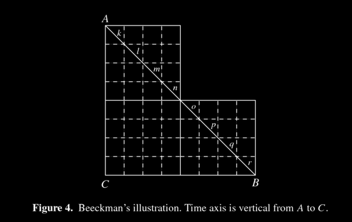
Figure of Beeckman (1618) showing a means to compute the area under a curve, in this example the line connecting points $A$ and $B$ . Using approximations by geometric figures with known area is the basis of Riemann sums.

Beeckman actually did more than find the area. He generalized the relationship of rate $\times$ time $=$ distance. The line was interpreting a velocity, the “squares”, then, provided an approximate distance traveled when the velocity is taken as a constant on the small time interval. Then the distance traveled can be approximated by a smaller quantity - just add the area of the rectangles squarely within the desired area ( $6 + 16 + 6$ ) - and a larger quantity - by including all rectangles that have a portion of their area within the desired area ( $10 + 16 + 10$ ). Beeckman argued that the error vanishes as the rectangles get smaller.

Adding up the smaller “squares” can be a bit more efficient if we were to add all those in a row, or column at once. We would then add the areas of a smaller number of rectangles. For this curve, the two approaches are basically identical. For other curves, identifying which squares in a row would be added is much more complicated (though useful), but for a curve generated by a function, identifying which “squares” go in a rectangle is quite easy, in fact we can see the rectangle’s area will be a base given by that of the squares, and height depending on the function.

36.1.1 Adding rectangles

The idea of the Riemann sum then is to approximate the area under the curve by the area of well-chosen rectangles in such a way that as the bases of the rectangles get smaller (hence adding more rectangles) the error in approximation vanishes.

Define a partition of $[a, b]$ to be a selection of points $a = x_{0} < x_{1} < \dots < x_{n - 1} < x_{n} = b$ . The norm of the partition is the largest of all the differences $| x_{i} - x_{i - 1} |$ . For a partition, consider an arbitrary selection of points $c_{i}$ satisfying $x_{i - 1} \leq c_{i} \leq x_{i}$ , $1 \leq i \leq n$ . Then the following is a Riemann sum:

$S_{n} = f (c_{1}) \cdot (x_{1} - x_{0}) + f (c_{2}) \cdot (x_{2} - x_{1}) + \dots + f (c_{n}) \cdot (x_{n} - x_{n - 1}) .$

Clearly for a given partition and choice of $c_{i}$ , the above can be computed. Each term $f (c_{i}) \cdot (x_{i} - x_{i - 1})$ can be visualized as the area of a rectangle with base spanning from $x_{i - 1}$ to $x_{i}$ and height given by the function value at $c_{i}$ . The following visualizes left Riemann sums for different values of $n$ in a way that makes Beekman’s intuition plausible – that as the number of rectangles gets larger, the approximate sum will get closer to the actual area.

To successfully compute a good approximation for the area, we would need to choose $c_{i}$ and the partition so that a formula can be found to express the dependence on the size of the partition.

For Archimedes’ problem - finding the area under $f (x) = x^{2}$ between $0$ and $1$ - if we take as a partition $x_{i} = i / n$ and $c_{i} = x_{i}$ , then the above sum becomes:

$\begin{aligned} S_{n} & = f (c_{1}) \cdot (x_{1} - x_{0}) + f (c_{2}) \cdot (x_{2} - x_{1}) + \dots + f (c_{n}) \cdot (x_{n} - x_{n - 1}) \\ = (x_{1})^{2} \cdot \frac{1}{n} + (x_{2})^{2} \cdot \frac{1}{n} + \dots + (x_{n})^{2} \cdot \frac{1}{n} \\ = 1^{2} \cdot \frac{1}{n^{3}} + 2^{2} \cdot \frac{1}{n^{3}} + \dots + n^{2} \cdot \frac{1}{n^{3}} \\ = \frac{1}{n^{3}} \cdot (1^{2} + 2^{2} + \dots + n^{2}) \\ = \frac{1}{n^{3}} \cdot \frac{n \cdot (n - 1) \cdot (2 n + 1)}{6} . \end{aligned}$

The latter uses a well-known formula for the sum of squares of the first $n$ natural numbers.

With this expression, it is readily seen that as $n$ gets large this value gets close to $2 / 6 = 1 / 3$ .

Note

The above approach, like Archimedes’, ends with a limit being taken. The answer comes from using a limit to add a big number of small values. As with all limit questions, worrying about whether a limit exists is fundamental. For this problem, we will see that for the general statement there is a stretching of the formal concept of a limit.

There is a more compact notation to $x_{1} + x_{2} + \dots + x_{n}$ , this using the summation notation or capital sigma. We have:

$Σ_{i = 1}^{n} x_{i} = x_{1} + x_{2} + \dots + x_{n}$

The notation includes three pieces of information:

The $Σ$ is an indication of a sum
The $i = 1$ and $n$ sub- and superscripts indicate the range to sum over.
The term $x_{i}$ is a general term describing the $i$ th entry, where it is understood that $i$ is just some arbitrary indexing value.

With this notation, a Riemann sum can be written as $Σ_{i = 1}^{n} f (c_{i}) (x_{i} - x_{i - 1})$ .

36.1.2 Other sums

The choice of the $c_{i}$ will give different answers for the approximation, though for an integrable function these differences will vanish in the limit. Some common choices are:

Using the right hand endpoint of the interval $[x_{i - 1}, x_{i}]$ giving the right-Riemann sum, $R_{n}$ .
The choice $c_{i} = x_{i - 1}$ gives the left-Riemann sum, $L_{n}$ .
The choice $c_{i} = (x_{i} + x_{i - 1}) / 2$ is the midpoint rule, $M_{n}$ .
If the function is continuous on the closed subinterval $[x_{i - 1}, x_{i}]$ , then it will take on its minimum and maximum values. By the extreme value theorem, we could take $c_{i}$ to correspond to either the maximum or the minimum. These choices give the “upper Riemann-sums” and “lower Riemann-sums”.

The choice of partition can also give different answers. A common choice is to break the interval into $n + 1$ equal-sized pieces. With $Δ = (b - a) / n$ , these pieces become the arithmetic sequence $a = a + 0 \cdot Δ < a + 1 \cdot Δ < a + 2 \cdot Δ < \dots < a + n \cdot Δ = b$ with $x_{i} = a + i (b - a) / n$ . (The range(a, b, length=n+1) command will compute these.) An alternate choice made below for one problem is to use a geometric progression:

$a = a (1 + α)^{0} < a (1 + α)^{1} < a (1 + α)^{2} < \dots < a (1 + α)^{n} = b .$

The general statement allows for any partition such that the largest gap goes to $0$ .

Riemann sums weren’t named after Riemann because he was the first to approximate areas using rectangles. Indeed, others had been using even more efficient ways to compute areas for centuries prior to Riemann’s work. Rather, Riemann put the definition of the area under the curve on a firm theoretical footing with the following theorem which gives a concrete notion of what functions are integrable:

Riemann Integral

A function $f$ is Riemann integrable over the interval $[a, b]$ and its integral will have value $V$ provided for every $ϵ > 0$ there exists a $δ > 0$ such that for any partition $a = x_{0} < x_{1} < \dots < x_{n} = b$ with $| x_{i} - x_{i - 1} | < δ$ and for any choice of points $x_{i - 1} \leq c_{i} \leq x_{i}$ this is satisfied:

$| \sum_{i = 1}^{n} f (c_{i}) (x_{i} - x_{i - 1}) - V | < ϵ .$

When the integral exists, it is written $V = \int_{a}^{b} f (x) d x$ .

History note

The expression $V = \int_{a}^{b} f (x) d x$ is known as the definite integral of $f$ over $[a, b]$ . Much earlier than Riemann, Cauchy had defined the definite integral in terms of a sum of rectangular products beginning with $S = (x_{1} - x_{0}) f (x_{0}) + (x_{2} - x_{1}) f (x_{1}) + \dots + (x_{n} - x_{n - 1}) f (x_{n - 1})$ (the left Riemann sum). He showed the limit was well defined for any continuous function. Riemann’s formulation relaxes the choice of partition and the choice of the $c_{i}$ so that integrability can be better understood.

36.1.3 Some immediate consequences

The following formulas are consequences when $f (x)$ is integrable. These mostly follow through a judicious rearranging of the approximating sums.

The area is $0$ when there is no width to the interval to integrate over:

$\int_{a}^{a} f (x) d x = 0.$

Even our definition of a partition doesn’t really apply, as we assume $a < b$ , but clearly if $a = x_{0} = x_{n} = b$ then our only”approximating” sum could be $f (a) (b - a) = 0$ .

The area under a constant function is found from the area of rectangle, a special case being $c = 0$ yielding $0$ area:

$\int_{a}^{b} c d x = c \cdot (b - a) .$

For any partition of $a < b$ , we have $S_{n} = c (x_{1} - x_{0}) + c (x_{2} - x_{1}) + \dots + c (x_{n} - x_{n - 1})$ . By factoring out the $c$ , we have a telescoping sum which means the sum simplifies to $S_{n} = c (x_{n} - x_{0}) = c (b - a)$ . Hence any limit must be this constant value.

Scaling the $y$ axis by a constant can be done before or after computing the area:

$\int_{a}^{b} c f (x) d x = c \int_{a}^{b} f (x) d x .$

Let $a = x_{0} < x_{1} < \dots < x_{n} = b$ be any partition. Then we have $S_{n} = c f (c_{1}) (x_{1} - x_{0}) + \dots + c f (c_{n}) (x_{n} - x_{n - 1})$ $=$ $c \cdot [f (c_{1}) (x_{1} - x_{0}) + \dots + f (c_{n}) (x_{n} - x_{n - 1})]$ . The “limit” of the left side is $\int_{a}^{b} c f (x) d x$ . The “limit” of the right side is $c \cdot \int_{a}^{b} f (x)$ . We call this a “sketch” as a formal proof would show that for any $ϵ$ we could choose a $δ$ so that any partition with norm $δ$ will yield a sum less than $ϵ$ . Here, then our “any” partition would be one for which the $δ$ on the left hand side applies. The computation shows that the same $δ$ would apply for the right hand side when $ϵ$ is the same.

The area is invariant under shifts left or right.

$\int_{a}^{b} f (x - c) d x = \int_{a - c}^{b - c} f (x) d x .$

Any partition $a = x_{0} < x_{1} < \dots < x_{n} = b$ is related to a partition of $[a - c, b - c]$ through $a - c < x_{0} - c < x_{1} - c < \dots < x_{n} - c = b - c$ . Let $d_{i} = c_{i} - c$ denote this partition, then we have:

$\begin{aligned} f (c_{1} - c) \cdot (x_{1} - x_{0}) & + f (c_{2} - c) \cdot (x_{2} - x_{1}) + \dots \\ + f (c_{n} - c) \cdot (x_{n} - x_{n - 1}) \\ = f (d_{1}) \cdot (x_{1} - c - (x_{0} - c)) + f (d_{2}) \cdot (x_{2} - c - (x_{1} - c)) + \dots \\ + f (d_{n}) \cdot (x_{n} - c - (x_{n - 1} - c)) . \end{aligned}$

The left side will have a limit of $\int_{a}^{b} f (x - c) d x$ the right would have a “limit” of $\int_{a - c}^{b - c} f (x) d x$ .

Similarly, reflections don’t effect the area under the curve, they just require a new parameterization:

$\int_{a}^{b} f (x) d x = \int_{- b}^{- a} f (- x) d x$

The scaling operation $g (x) = f (c x)$ has the following:

$\int_{a}^{b} f (c \cdot x) d x = \frac{1}{c} \int_{c a}^{c b} f (x) d x$

The scaling operation shifts $a$ to $c a$ and $b$ to $c b$ so the limits of integration make sense. However, the area stretches by $c$ in the $x$ direction, so must contract by $c$ in the $y$ direction to stay in balance. Hence the factor of $1 / c$ .

Combining two operations above, the operation $g (x) = \frac{1}{h} f (\frac{x - c}{h})$ will leave the area between $a$ and $b$ under $g$ the same as the area under $f$ between $(a - c) / h$ and $(b - c) / h$ .

The area between $a$ and $b$ can be broken up into the sum of the area between $a$ and $c$ and that between $c$ and $b$ .

$\int_{a}^{b} f (x) d x = \int_{a}^{c} f (x) d x + \int_{c}^{b} f (x) d x .$

For this, suppose we have a partition for both the integrals on the right hand side for a given $ϵ / 2$ and $δ$ . Combining these into a partition of $[a, b]$ will mean $δ$ is still the norm. The approximating sum will combine to be no more than $ϵ / 2 + ϵ / 2$ , so for a given $ϵ$ , this $δ$ applies.

This is due to the area on the left and right of $0$ being equivalent.

The “reversed” area is the same, only accounted for with a minus sign.

$\int_{a}^{b} f (x) d x = - \int_{b}^{a} f (x) d x .$

A consequence of the last few statements is:

If $f (x)$ is an even function, then $\int_{- a}^{a} f (x) d x = 2 \int_{0}^{a} f (x) d x$ . If $f (x)$ is an odd function, then $\int_{- a}^{a} f (x) d x = 0$ .

If $g$ bounds $f$ then the area under $g$ will bound the area under $f$ , in particular if $f (x)$ is non negative, so will the area under $f$ be non negative for any $a < b$ . (This assumes that $g$ and $f$ are integrable.)

If $0 \leq f (x) \leq g (x)$ then $\int_{a}^{b} f (x) d x \leq \int_{a}^{b} g (x) d x .$

For any partition of $[a, b]$ and choice of $c_{i}$ , we have the term-by-term bound $f (c_{i}) (x_{i} - x_{i - 1}) \leq g (c_{i}) (x_{i} - x_{i - 1})$ So any sequence of partitions that converges to the limits will have this inequality maintained for the sum.

36.1.4 Some known integrals

Using the definition, we can compute a few definite integrals:

$\int_{a}^{b} c d x = c \cdot (b - a) .$

$\int_{a}^{b} x d x = \frac{b^{2}}{2} - \frac{a^{2}}{2} .$

This is just the area of a trapezoid with heights $a$ and $b$ and side length $b - a$ , or $1 / 2 \cdot (b + a) \cdot (b - a)$ . The right sum would be:

$\begin{aligned} S & = x_{1} \cdot (x_{1} - x_{0}) + x_{2} \cdot (x_{2} - x_{1}) + \dots x_{n} \cdot (x_{n} - x_{n - 1}) \\ = (a + 1 \frac{b - a}{n}) \cdot \frac{b - a}{n} + (a + 2 \frac{b - a}{n}) \cdot \frac{b - a}{n} + \dots (a + n \frac{b - a}{n}) \cdot \frac{b - a}{n} \\ = n \cdot a \cdot (\frac{b - a}{n}) + (1 + 2 + \dots n) \cdot (\frac{b - a}{n})^{2} \\ = n \cdot a \cdot (\frac{b - a}{n}) + \frac{n (n + 1)}{2} \cdot (\frac{b - a}{n})^{2} \\ \to a \cdot (b - a) + \frac{(b - a)^{2}}{2} \\ = \frac{b^{2}}{2} - \frac{a^{2}}{2} . \end{aligned}$

$\int_{a}^{b} x^{2} d x = \frac{b^{3}}{3} - \frac{a^{3}}{3} .$

This is similar to the Archimedes case with $a = 0$ and $b = 1$ shown above.

$\int_{a}^{b} x^{k} d x = \frac{b^{k + 1}}{k + 1} - \frac{a^{k + 1}}{k + 1}, k \neq - 1$

.

Cauchy showed this using a geometric series for the partition, not the arithmetic series $x_{i} = a + i (b - a) / n$ . The series defined by $1 + α = (b / a)^{1 / n}$ , then $x_{i} = a \cdot (1 + α)^{i}$ . Here the bases $x_{i + 1} - x_{i}$ simplify to $x_{i} \cdot α$ and $f (x_{i}) = (a \cdot (1 + α)^{i})^{k} = a^{k} (1 + α)^{i k}$ , or $f (x_{i}) (x_{i + 1} - x_{i}) = a^{k + 1} α [(1 + α)^{k + 1}]^{i}$ , so, using $u = (1 + α)^{k + 1} = (b / a)^{(k + 1) / n}$ , $f (x_{i}) \cdot (x_{i + 1} - x_{i}) = a^{k + 1} α u^{i}$ . This gives

$\begin{aligned} S & = a^{k + 1} α u^{0} + a^{k + 1} α u^{1} + \dots + a^{k + 1} α u^{n - 1} \\ = a^{k + 1} \cdot α \cdot (u^{0} + u^{1} + \cdot u^{n - 1}) \\ = a^{k + 1} \cdot α \cdot \frac{u^{n} - 1}{u - 1} \\ = (b^{k + 1} - a^{k + 1}) \cdot \frac{α}{(1 + α)^{k + 1} - 1} \\ \to \frac{b^{k + 1} - a^{k + 1}}{k + 1} . \end{aligned}$

$\int_{a}^{b} x^{- 1} d x = \log (b) - \log (a), (0 < a < b) .$

Again, Cauchy showed this using a geometric series. The expression $f (x_{i}) \cdot (x_{i + 1} - x_{i})$ becomes just $α$ . So the approximating sum becomes:

$S = f (x_{0}) (x_{1} - x_{0}) + f (x_{1}) (x_{2} - x_{1}) + \dots + f (x_{n - 1}) (x_{n} - x_{n - 1}) = α + α + \dots α = n α .$

But, letting $x = 1 / n$ , the limit above is just the limit of

$lim_{x \to 0 +} \frac{(b / a)^{x} - 1}{x} = \log (b / a) = \log (b) - \log (a) .$

(Using L’Hopital’s rule to compute the limit.)

Certainly other integrals could be computed with various tricks, but we won’t pursue this. There is another way to evaluate integrals using the forthcoming Fundamental Theorem of Calculus.

36.1.5 Some other consequences

The definition is defined in terms of any partition with its norm bounded by $δ$ . If you know a function $f$ is Riemann integrable, then it is enough to consider just a regular partition $x_{i} = a + i \cdot (b - a) / n$ when forming the sums, as was done above. It is just that showing a limit for just this particular type of partition would not be sufficient to prove Riemann integrability.
The choice of $c_{i}$ is arbitrary to allow for maximum flexibility. The Darboux integrals use the maximum and minimum over the subinterval. It is sufficient to prove integrability to show that the limit exists with just these choices.
Most importantly,

A continuous function on $[a, b]$ is Riemann integrable on $[a, b]$ .

The main idea behind this is that the difference between the maximum and minimum values over a partition gets small. That is if $[x_{i - 1}, x_{i}]$ is like $1 / n$ is length, then the difference between the maximum of $f$ over this interval, $M$ , and the minimum, $m$ over this interval will go to zero as $n$ gets big. That $m$ and $M$ exists is due to the extreme value theorem, that this difference goes to $0$ is a consequence of continuity. What is needed is that this value goes to $0$ at the same rate – no matter what interval is being discussed – is a consequence of a notion of uniform continuity, a concept discussed in advanced calculus, but which holds for continuous functions on closed intervals. Armed with this, the Riemann sum for a general partition can be bounded by this difference times $b - a$ , which will go to zero. So the upper and lower Riemann sums will converge to the same value.

A “jump”, or discontinuity of the first kind, is a value $c$ in $[a, b]$ where $lim_{x \to c +} f (x)$ and $lim_{x \to c -} f (x)$ both exist, but are not equal. It is true that a function that is not continuous on $I = [a, b]$ , but only has discontinuities of the first kind on $I$ will be Riemann integrable on $I$ .

For example, the function $f (x) = 1$ for $x$ in $[0, 1]$ and $0$ otherwise will be integrable, as it is continuous at all but two points, $0$ and $1$ , where it jumps.

Some functions can have infinitely many points of discontinuity and still be integrable. The example of $f (x) = 1 / q$ when $x = p / q$ is rational, and $0$ otherwise is often used as an example.

36.2 Numeric integration

The Riemann sum approach gives a method to approximate the value of a definite integral. We just compute an approximating sum for a large value of $n$ , so large that the limiting value and the approximating sum are close.

To see the mechanics, let’s again return to Archimedes’ problem and compute $\int_{0}^{1} x^{2} d x$ .

Let us fix some values:

a, b = 0, 1
f(x) = x^2

f (generic function with 1 method)

Then for a given $n$ we have some steps to do: create the partition, find the $c_{i}$ , multiply the pieces and add up. Here is one way to do all this:

n = 5
xs = a:(b-a)/n:b       # also range(a, b, length=n)
deltas = diff(xs)      # forms x2-x1, x3-x2, ..., xn-xn-1
cs = xs[1:end-1]       # finds left-hand end points. xs[2:end] would be right-hand ones.

0.0:0.2:0.8

Now to multiply the values. We want to sum the product f(cs[i]) * deltas[i], here is one way to do so:

sum(f(cs[i]) * deltas[i] for i in 1:length(deltas))

0.24000000000000002

Our answer is not so close to the value of $1 / 3$ , but what did we expect - we only used $n = 5$ intervals. Trying again with $50, 000$ gives us:

n = 50_000
xs = a:(b-a)/n:b
deltas = diff(xs)
cs = xs[1:end-1]
sum(f(cs[i]) * deltas[i] for i in 1:length(deltas))

0.3333233333999998

This value is about $10^{- 5}$ off from the actual answer of $1 / 3$ .

We should expect that larger values of $n$ will produce better approximate values, as long as numeric issues don’t get involved.

Before continuing, we define a function to compute Riemann sums for us with an extra argument to specifying one of four methods for computing $c_{i}$ :

riemann(f, a, b, n; method="right") = riemann(f, range(a,b,n+1); method=method)
function riemann(f, xs; method="right")
    Ms = (left = (f,a,b) -> f(a),
          right= (f,a,b) -> f(b),
          trapezoid = (f,a,b) -> (f(a) + f(b))/2,
          simpsons  = (f,a,b) -> (c = a/2 + b/2; (1/6) * (f(a) + 4*f(c) + f(b))),
          )
    _riemann(Ms[Symbol(method)], f, xs)
end
function _riemann(M, f, xs)
    xs′ = zip(xs[1:end-1], xs[2:end])
    sum(M(f, a, b) * (b-a) for (a,b) ∈ xs′)
end

(This function is defined in CalculusWithJulia and need not be copied over if that package is loaded.)

With this, we can easily find an approximate answer. We wrote the function to use the familiar template action(function, arguments...), so we pass in a function and arguments to describe the problem (a, b, and n and, optionally, the method):

f(x) = exp(x)
riemann(f, 0, 5, 10)   # S_10

187.324835773627

Or with more intervals in the partition

riemann(f, 0, 5, 50_000)

147.42052988337647

(The answer is $e^{5} - e^{0} = 147.4131591025766 \dots$ , which shows that even $50, 000$ partitions is not enough to guarantee many digits of accuracy.)

36.3 “Negative” area

So far, we have had the assumption that $f (x) \geq 0$ , as that allows us to define the concept of area. We can define the signed area between $f (x)$ and the $x$ axis through the definite integral:

$A = \int_{a}^{b} f (x) d x .$

The right hand side is defined whenever the Riemann limit exists and in that case we call $f (x)$ Riemann integrable. (The definition does not suppose $f$ is non-negative.)

Suppose $f (a) = f (b) = 0$ for $a < b$ and for all $a < x < b$ we have $f (x) < 0$ . Then we can see easily from the geometry (or from the Riemann sum approximation) that

$\int_{a}^{b} f (x) d x = - \int_{a}^{b} | f (x) | d x .$

If we think of the area below the $x$ axis as “signed” area carrying a minus sign, then the total area can be seen again as a sum, only this time some of the summands may be negative.

Example

Consider a function $g (x)$ defined through its piecewise linear graph:

Compute $\int_{- 3}^{- 1} g (x) d x$ . The area comprised of a square of area $1$ and a triangle with area $1 / 2$ , so should be $3 / 2$ .
Compute $\int_{- 3}^{0} g (x) d x$ . In addition to the above, there is a triangle with area $1 / 2$ , but since the function is negative, this area is added in as $- 1 / 2$ . In total then we have $1 + 1 / 2 - 1 / 2 = 1$ for the answer.
Compute $\int_{- 3}^{1} g (x) d x$ :

We could add the signed area over $[0, 1]$ to the above, but instead see a square of area $1$ , a triangle with area $1 / 2$ and a triangle with signed area $- 1$ . The total is then $1 / 2$ .

Compute $\int_{- 3}^{3} g (x) d x$ :

We could add the area, but let’s use a symmetry trick. This is clearly twice our second answer, or $2$ . (This is because $g (x)$ is an even function, as we can tell from the graph.)

Example

Suppose $f (x)$ is an odd function, then $f (x) = - f (- x)$ for any $x$ . So the signed area between $[- a, 0]$ is related to the signed area between $[0, a]$ but of different sign. This gives $\int_{- a}^{a} f (x) d x = 0$ for odd functions.

An immediate consequence would be $\int_{- π}^{π} \sin (x) = 0$ , as would $\int_{- a}^{a} x^{k} d x$ for any odd integer $k > 0$ .

Example

Numerically estimate the definite integral $\int_{0}^{e} x \log (x) d x$ . (We redefine the function to be $0$ at $0$ , so it is continuous.)

We have to be a bit careful with the Riemann sum, as the left Riemann sum will have an issue at $0 = x_{0}$ (0*log(0)) returns NaN which will poison any subsequent arithmetic operations, so the value returned will be NaN and not an approximate answer. We could define our function with a check:

h(x) = x > 0 ? x * log(x) : 0.0

h (generic function with 1 method)

This is actually inefficient, as the check for the size of x will slow things down a bit. Since we will call this function 50,000 times, we would like to avoid this, if we can. In this case just using the right sum will work:

h(x) = x * log(x)
riemann(h, 0, 2, 50_000, method="right")

0.38632208884775826

(The default is "right", so no method specified would also work.)

Example

Let $j (x) = \sqrt{1 - x^{2}}$ . The area under the curve between $- 1$ and $1$ is $π / 2$ . Using a Riemann sum with 4 equal subintervals and the midpoint, estimate $π$ . How close are you?

The partition is $- 1 < - 1 / 2 < 0 < 1 / 2 < 1$ . The midpoints are $- 3 / 4, - 1 / 4, 1 / 4, 3 / 4$ . We thus have that $π / 2$ is approximately:

xs = range(-1, 1, length=5)
deltas = diff(xs)
cs = [-3/4, -1/4, 1/4, 3/4]
j(x) = sqrt(1 - x^2)
a = sum(j(c)*delta for (c,delta) in zip(cs, deltas))
a, pi/2  # π ≈  2a

(1.629683664318002, 1.5707963267948966)

(For variety, we used an alternate way to sum over two vectors.)

So $π$ is about 2a.

Example

We have the well-known triangle inequality which says for an individual sum: $| a + b | \leq | a | + | b |$ . Applying this recursively to a partition with $a < b$ gives:

$\begin{matrix} | f (c_{1}) (x_{1} - x_{0}) + f (c_{2}) (x_{2} - x_{1}) + \dots + f (c_{n}) (x_{n} - x_{1}) | \\ \leq | f (c_{1}) (x_{1} - x_{0}) | + | f (c_{2}) (x_{2} - x_{1}) | + \dots + | f (c_{n}) (x_{n} - x_{n - 1}) | \\ = | f (c_{1}) | (x_{1} - x_{0}) + | f (c_{2}) | (x_{2} - x_{1}) + \dots + | f (c_{n}) | (x_{n} - x_{n - 1}) . \end{matrix}$

This suggests that the following inequality holds for integrals:

$| \int_{a}^{b} f (x) d x | \leq \int_{a}^{b} | f (x) | d x$ .

This can be used to give bounds on the size of an integral. For example, suppose you know that $f (x)$ is continuous on $[a, b]$ and takes its maximum value of $M$ and minimum value of $m$ . Letting $K$ be the larger of $| M |$ and $| m |$ , gives this bound when $a < b$ :

$| \int_{a}^{b} f (x) d x | \leq \int_{a}^{b} | f (x) | d x \leq \int_{a}^{b} K d x = K (b - a) .$

While such bounds are disappointing, often, when looking for specific values, they are very useful when establishing general truths, such as is done with proofs.

36.4 Error estimate

The Riemann sum above is actually extremely inefficient. To see how much, we can derive an estimate for the error in approximating the value using an arithmetic progression as the partition. Let’s assume that our function $f (x)$ is increasing, so that the right sum gives an upper estimate and the left sum a lower estimate, so the error in the estimate will be between these two values:

$\begin{aligned} error & \leq [f (x_{1}) \cdot (x_{1} - x_{0}) + f (x_{2}) \cdot (x_{2} - x_{1}) + \dots + f (x_{n - 1}) (x_{n - 1} - x_{n - 2}) + f (x_{n}) \cdot (x_{n} - x_{n - 1})] \\ - [f (x_{0}) \cdot (x_{1} - x_{0}) + f (x_{1}) \cdot (x_{2} - x_{1}) + \dots + f (x_{n - 1}) (x_{n} - x_{n - 1})] \\ = \frac{b - a}{n} \cdot ([f (x_{1}) + f (x_{2}) + \dots + f (x_{n})] - [f (x_{0}) + \dots + f (x_{n - 1})]) \\ = \frac{b - a}{n} \cdot (f (b) - f (a)) . \end{aligned}$

We see the error goes to $0$ at a rate of $1 / n$ with the constant depending on $b - a$ and the function $f$ . In general, a similar bound holds when $f$ is not monotonic.

There are other ways to approximate the integral that use fewer points in the partition. Simpson’s rule is one, where instead of approximating the area with rectangles that go through some $c_{i}$ in $[x_{i - 1}, x_{i}]$ instead the function is approximated by the quadratic polynomial going through $x_{i - 1}$ , $(x_{i} + x_{i - 1}) / 2$ , and $x_{i}$ and the exact area under that polynomial is used in the approximation. The explicit formula is:

$A \approx \frac{b - a}{3 n} (f (x_{0}) + 4 f (x_{1}) + 2 f (x_{2}) + 4 f (x_{3}) + \dots + 2 f (x_{n - 2}) + 4 f (x_{n - 1}) + f (x_{n})) .$

The error in this approximation can be shown to be

$error \leq \frac{(b - a)^{5}}{180 n^{4}} {max}_{ξ in [a, b]} | f^{(4)} (ξ) | .$

That is, the error is like $1 / n^{4}$ with constants depending on the length of the interval, $(b - a)^{5}$ , and the maximum value of the fourth derivative over $[a, b]$ . This is significant, the error in $10$ steps of Simpson’s rule is on the scale of the error of $10, 000$ steps of the Riemann sum for well-behaved functions.

Note

The Wikipedia article mentions that Kepler used a similar formula $100$ years prior to Simpson, or about $200$ years before Riemann published his work. Again, the value in Riemann’s work is not the computation of the answer, but the framework it provides in determining if a function is Riemann integrable or not.

36.5 Gauss quadrature

The formula for Simpson’s rule was the composite formula. If just a single rectangle is approximated over $[a, b]$ by a parabola interpolating the points $x_{1} = a$ , $x_{2} = (a + b) / 2$ , and $x_{3} = b$ , the formula is:

$\frac{b - a}{6} (f (x_{1}) + 4 f (x_{2}) + f (x_{3})) .$

This formula will actually be exact for any 3rd degree polynomial. In fact an entire family of similar approximations using $n$ points can be made exact for any polynomial of degree $n - 1$ or lower. But with non-evenly spaced points, even better results can be found.

The formulas for an approximation to the integral $\int_{- 1}^{1} f (x) d x$ discussed so far can be written as:

$\begin{aligned} S & = f (x_{1}) Δ_{1} + f (x_{2}) Δ_{2} + \dots + f (x_{n}) Δ_{n} \\ = w_{1} f (x_{1}) + w_{2} f (x_{2}) + \dots + w_{n} f (x_{n}) . \end{aligned}$

The $w$ s are “weights” and the $x$ s are nodes. A Gaussian quadrature rule is a set of weights and nodes for $i = 1, \dots n$ for which the sum is exact for any $f$ which is a polynomial of degree $2 n - 1$ or less. Such choices then also approximate well the integrals of functions which are not polynomials of degree $2 n - 1$ , provided $f$ can be well approximated by a polynomial over $[- 1, 1]$ . (Which is the case for the “nice” functions we encounter.) Some examples are given in the questions.

36.5.1 The quadgk function

In Julia a modification of the Gauss quadrature rule is implemented in the quadgk function (from the QuadGK package) to give numeric approximations to integrals. The quadgk function also has the familiar interface action(function, arguments...). Unlike our riemann function, there is no n specified, as the number of steps is adaptively determined. (There is more partitioning occurring where the function is changing rapidly.) Instead, the algorithm outputs an estimate on the possible error along with the answer. Instead of $n$ , some trickier problems require a specification of an error threshold.

To use the function, we have:

f(x) = x * log(x)
quadgk(f, 0, 2)

(0.38629436103070175, 4.856575112145755e-9)

As mentioned, there are two values returned: an approximate answer, and an error estimate. In this example we see that the value of $0.3862943610307017$ is accurate to within $10^{- 9}$ . (The actual answer is $- 1 + 2 \cdot \log (2)$ and the error is only $10^{- 11}$ . The reported error is an upper bound, and may be conservative, as with this problem.) Our previous answer using $50, 000$ right-Riemann sums was $0.38632208884775737$ and is only accurate to $10^{- 5}$ . By contrast, this method uses just $256$ function evaluations in the above problem.

The method should be exact for polynomial functions:

f(x) = x^5 - x + 1
quadgk(f, -2, 2)

(3.9999999999999973, 1.3322676295501878e-15)

The error term is $0$ , answer is $4$ up to the last unit of precision (1 ulp), so any error is only in floating point approximations.

For the numeric computation of definite integrals, the quadgk function should be used over the Riemann sums or even Simpson’s rule.

Here are some sample integrals computed with quadgk:

$\int_{0}^{π} \sin (x) d x$

quadgk(sin, 0, pi)

(2.0000000000000004, 1.7901236049056024e-12)

(Again, the actual answer is off only in the last digit, the error estimate is an upper bound.)

$\int_{0}^{2} x^{x} d x$

u(x) = x^x
quadgk(u, 0, 2)

(2.8338767448900546, 1.948175154531384e-8)

$\int_{0}^{5} e^{x} d x$

quadgk(exp, 0, 5)

(147.41315910257657, 2.6594506152832764e-8)

When composing the answer with other functions it may be desirable to drop the error in the answer. Two styles can be used for this. The first is to just name the two returned values:

A, err = quadgk(cos, 0, pi/4)
A

0.7071067811865475

The second is to ask for just the first component of the returned value:

A = quadgk(tan, 0, pi/4)[1] # or first(quadgk(tan, 0, pi/4))

0.3465735902799726

To visualize the choice of nodes by the algorithm, we have for $f (x) = \sin (x)$ over $[0, π]$ relatively few nodes used to get a high-precision estimate:

For a more oscillatory function, more nodes are chosen:

Example

In probability theory, a univariate density is a function, $f (x)$ such that $f (x) \geq 0$ and $\int_{a}^{b} f (x) d x = 1$ , where $a$ and $b$ are the range of the distribution. The Von Mises distribution, takes the form

$k (x) = C \cdot \exp (\cos (x)), - π \leq x \leq π$

Compute $C$ (numerically).

The fact that $1 = \int_{- π}^{π} C \cdot \exp (\cos (x)) d x = C \int_{- π}^{π} \exp (\cos (x)) d x$ implies that $C$ is the reciprocal of

k(x) = exp(cos(x))
A,err = quadgk(k, -pi, pi)

(7.954926521012919, 3.9023298370466364e-8)

C = 1/A
k₁(x) = C * exp(cos(x))

k₁ (generic function with 1 method)

The cumulative distribution function for $k (x)$ is $K (x) = \int_{- π}^{x} k (u) d u$ , $- π \leq x \leq π$ . We just showed that $K (π) = 1$ and it is trivial that $K (- π) = 0$ . The quantiles of the distribution are the values $q_{1}$ , $q_{2}$ , and $q_{3}$ for which $K (q_{i}) = i / 4$ . Can we find these?

First we define a function, that computes $K (x)$ :

K(x) = quadgk(k₁, -pi, x)[1]

K (generic function with 1 method)

(The trailing [1] is so only the answer - and not the error - is returned.)

The question asks us to solve $K (x) = 0.25$ , $K (x) = 0.5$ and $K (x) = 0.75$ . The Roots package can be used for such work, in particular find_zero. We will use a bracketing method, as clearly $K (x)$ is increasing, as $k (u)$ is positive, so we can just bracket our answer with $- π$ and $π$ . (We solve $K (x) - p = 0$ , so $K (π) - p > 0$ and $K (- π) - p < 0$ .). We could do this with [find_zero(x -> K(x) - p, (-pi, pi)) for p in [0.25, 0.5, 0.75]], but that is a bit less performant than using the solve interface for this task:

Z = ZeroProblem((x,p) -> K(x) - p, (-pi, pi))
solve.(Z, (1/4, 1/2, 3/4))

(-0.8097673745015915, 0.0, 0.8097673745016285)

The middle one is clearly $0$ . This distribution is symmetric about $0$ , so half the area is to the right of $0$ and half to the left, so clearly when $p = 0.5$ , $x$ is $0$ . The other two show that the area to the left of $- 0.809767$ is equal to the area to the right of $0.809767$ and equal to $0.25$ .

Example: Gauss nodes

The QuadGK.gauss(n) function returns a pair of $n$ quadrature points and weights to integrate a function over the interval $(- 1, 1)$ , with an option to use a different interval $(a, b)$ . For a given $n$ , these values exactly integrate any polynomial of degree $2 n - 1$ or less. The pattern to integrate below can be expressed in other ways, but this is intended to be direct:

xs, ws = QuadGK.gauss(5)

([-0.906179845938664, -0.5384693101056831, 0.0, 0.5384693101056831, 0.906179845938664], [0.2369268850561892, 0.4786286704993663, 0.5688888888888887, 0.4786286704993663, 0.2369268850561892])

f(x) = exp(cos(x))
sum(w * f(x) for (x, w) in zip(xs, ws))

4.68315881456892

The zip function is used to iterate over the xs and ws as pairs of values.

36.6 Questions

Question

Using geometry, compute the definite integral:

$\int_{- 5}^{5} \sqrt{5^{2} - x^{2}} d x .$

Question

Using geometry, compute the definite integral:

$\int_{- 2}^{2} (2 - | x |) d x$

Question

Using geometry, compute the definite integral:

$\int_{0}^{3} 3 d x + \int_{3}^{9} (3 + 3 (x - 3)) d x$

Question

Using geometry, compute the definite integral:

$\int_{0}^{5} ⌊ x ⌋ d x$

(The notation $⌊ x ⌋$ is the integer such that $⌊ x ⌋ \leq x < ⌊ x ⌋ + 1$ .)

Question

Using geometry, compute the definite integral between $- 3$ and $3$ of this graph comprised of lines and circular arcs:

The value is:

Question

For the function $f (x) = \sin (π x)$ , estimate the integral for $- 1$ to $1$ using a left-Riemann sum with the partition $- 1 < - 1 / 2 < 0 < 1 / 2 < 1$ .

Question

Without doing any real work, find this integral:

$\int_{- π / 4}^{π / 4} \tan (x) d x .$

Question

Without doing any real work, find this integral:

$\int_{3}^{5} (1 - | x - 4 |) d x$

Question

Suppose you know that for the integrable function $\int_{a}^{b} f (u) d u = 1$ and $\int_{a}^{c} f (u) d u = p$ . If $a < c < b$ what is $\int_{c}^{b} f (u) d u$ ?

Question

What is $\int_{0}^{2} x^{4} d x$ ? Use the rule for integrating $x^{n}$ .

Question

Solve for a value of $x$ for which:

$\int_{1}^{x} \frac{1}{u} d u = 1.$

Question

Solve for a value of $n$ for which

$\int_{0}^{1} x^{n} d x = \frac{1}{12} .$

Question

Suppose $f (x) > 0$ and $a < c < b$ . Define $F (x) = \int_{a}^{x} f (u) d u$ . What can be said about $F (b)$ and $F (c)$ ?

Question

For the right Riemann sum approximating $\int_{0}^{10} e^{x} d x$ with $n = 100$ subintervals, what would be a good estimate for the error?

Question

Use quadgk to find the following definite integral:

$\int_{1}^{4} x^{x} d x .$

Question

Use quadgk to find the following definite integral:

$\int_{0}^{3} e^{- x^{2}} d x .$

Question

Use quadgk to find the following definite integral:

$\int_{0}^{9 / 10} \tan (u \frac{π}{2}) d u .$

Question

Use quadgk to find the following definite integral:

$\int_{- 1 / 2}^{1 / 2} \frac{1}{\sqrt{1 - x^{2}}} d x$

Question

0,0

n = 2.00

Riemann sum=0.1287

JXG = require("jsxgraph");

b = JXG.JSXGraph.initBoard('jsxgraph', {
    boundingbox: [-0.5,0.3,1.5,-1/4], axis:true
});

g = function(x) { return x*x*x*x +  10*x*x - 60* x + 100}
f = function(x) {return 1/Math.sqrt(g(x))};

type = "right";
l = 0;
r = 1;
rsum = function() {
    return JXG.Math.Numerics.riemannsum(f,n.Value(), type, l, r);
};
n =   b.create('slider', [[0.1, -0.05],[0.75,-0.05], [2,1,50]],{name:'n',snapWidth:1});

graph = b.create('functiongraph', [f, l, r]);
os = b.create('riemannsum',
                  [f,
                   function(){ return n.Value();},
                   type, l, r
                  ],
                  {fillColor:'#ffff00', fillOpacity:0.3});

b.create('text', [0.1,0.25, function(){
    return 'Riemann sum='+(rsum().toFixed(4));
}]);

The interactive graphic shows the area of a right-Riemann sum for different partitions. The function is

$f (x) = \frac{1}{\sqrt{x^{4} + 10 x^{2} - 60 x + 100}}$

When $n = 5$ what is the area of the Riemann sum?

When $n = 50$ what is the area of the Riemann sum?

Using quadgk what is the area under the curve?

Question

Gauss nodes for approximating the integral $\int_{- 1}^{1} f (x) d x$ for $n = 4$ are:

ns = [-0.861136, -0.339981, 0.339981, 0.861136]

4-element Vector{Float64}:
 -0.861136
 -0.339981
  0.339981
  0.861136

The corresponding weights are

wts = [0.347855, 0.652145, 0.652145, 0.347855]

4-element Vector{Float64}:
 0.347855
 0.652145
 0.652145
 0.347855

Use these to estimate the integral $\int_{- 1}^{1} \cos (π / 2 \cdot x) d x$ with $w_{1} f (x_{1}) + w_{2} f (x_{2}) + w_{3} f (x_{3}) + w_{4} f (x_{4})$ .

The actual answer is $4 / π$ . How far off is the approximation based on 4 points?

Question

Using the Gauss nodes and weights from the previous question, estimate the integral of $f (x) = e^{x}$ over $[- 1, 1]$ . The value is: