using CalculusWithJulia
using Plots
plotly()
using QuadGK
using SymPy
using HCubature
import ImplicitIntegration63 Multi-dimensional integrals
This section uses these add-on packages:
The definition of the definite integral, \(\int_a^b f(x)dx\), is based on Riemann sums.
We review, using a more general form than previously. Consider a bounded function \(f\) over \([a,b]\). A partition, \(P\), is based on \(a = x_0 < x_1 < \cdots < x_n = b\). For each subinterval \([x_{i-1}, x_{i}]\) take \(m_i(f) = \inf_{u \text{ in } [x_{i-1},x_i]} f(u)\) and \(M_i(f) = \sup_{u \text{ in } [x_{i-1},x_i]} f(u)\). (When \(f\) is continuous, \(m_i\) and \(M_i\) are realized at points of \([x_{i-1},x_i]\), though that isn’t assumed here. The use of “\(\sup\)” and “\(\inf\)” is a mathematically formal means to replace this in general.) Let \(\Delta x_i = x_i - x_{i-1}\). Form the sums \(m(f, P) = \sum_i m_i(f) \Delta x_i\) and \(M(f, P) = \sum_i M_i(f) \Delta x_i\). These are the lower and upper Riemann sums for a partition. A general Riemann sum would be formed by selecting \(c_i\) from \([x_{i-1}, x_i]\) and forming \(S(f,P) = \sum f(c_i) \Delta x_i\). It will be the case that \(m(f,P) \leq S(f,P) \leq M(f,P)\), as this is true for each sub-interval of the partition.
If, as the largest diameter (\(\Delta x_i\)) of the partition \(P\) goes to \(0\), the upper and lower sums converge to the same limit, then \(f\) is called Riemann integrable over \([a,b]\). If \(f\) is Riemann integrable, any Riemann sum will converge to the definite integral as the partitioning shrinks.
Continuous functions are known to be Riemann integrable, as are functions with only finitely many discontinuities, though this isn’t the most general case of integrable functions, which will be stated below.
In practice, we don’t typically compute integrals using a limit of a partition, though the approach may provide direction to numeric answers, as the Fundamental Theorem of Calculus relates the definite integral with an antiderivative of the integrand.
The multidimensional case will prove to be similar where a Riemann sum is used to define the value being discussed, but a theorem of Fubini will allow the computation of integrals using the Fundamental Theorem of Calculus.
63.1 Integration theory

The definition of the multi-dimensional integral is more involved than the one-dimensional case due to the possibly increased complexity of the region. This will require additional steps. The basic approach is as follows.
First, let \(R = [a_1, b_1] \times [a_2, b_2] \times \cdots \times [a_n, b_n]\) be a closed rectangular region. If \(n=2\), this is a rectangle, and if \(n=3\), a box. We begin by defining integration over closed rectangular regions. For each side, a partition \(P_i\) is chosen based on \(a_i = x_{i0} < x_{i1} < \cdots < x_{ik} = b_i\). Then a sub-rectangular region would be of the form \(R' = P_{1j_1} \times P_{2j_2} \times \cdots \times P_{nj_n}\), where \(P_{ij_i}\) is one of the partitioning sub intervals of \([a_i, b_i]\). Set \(\Delta R' = \Delta P_{1j_1} \cdot \Delta P_{2j_2} \cdot\cdots\cdot\Delta P_{nj_n}\) to be the \(n\)-dimensional volume of the sub-rectangular region.
For each sub-rectangular region, we can define \(m(f,R')\) to be \(\inf_{u \text{ in } R'} f(u)\) and \(M(f, R') = \sup_{u \text{ in } R'} f(u)\). If we enumerate all the sub-rectangular regions, we can define \(m(f, P) = \sum_i m(f, R_i) \Delta R_i\) and \(M(f,P) = \sum_i M(f, R_i)\Delta R_i\), as in the one-dimensional case. These are upper and lower sums, and, as before, would bound the Riemann sum formed by choosing any \(c_i\) in \(R_i\) and computing \(S(f,P) = \sum_i f(c_i) \Delta R_i\).
As with the one-dimensional case, \(f\) is Riemann integrable over \(R\) if the limits of \(m(f,P)\) and \(M(f,P)\) exist and are identical as the diameter of the partition (defined as the largest diameter of each side) goes to \(0\). If the limits are equal, then so is the limit of any Riemann sum.
When \(f\) is Riemann integrable over a rectangular region \(R\), we denote the limit by any of:
\[ \iint_R f(x) dV, \quad \iint_R fdV, \quad \iint_R f(x_1, \dots, x_n) dx_1 \cdot\cdots\cdot dx_n, \quad\iint_R f(\vec{x}) d\vec{x}. \]
A key fact, requiring proof, is:
Any continuous function, \(f\), is Riemann integrable over a closed, bounded rectangular region.
As with one-dimensional integrals, from the Riemann sum definition, several familiar properties for integrals follow. Let \(V(R)\) be the volume of \(R\) found by multiplying the side-lengths together.
Constants:
- A constant is Riemann integrable and: \(\iint_R c dV = c V(R)\).
Linearity:
- For integrable \(f\) and \(g\) and constants \(a\) and \(b\):
\[ \iint_R (af(x) + bg(x))dV = a\iint_R f(x)dV + b\iint_R g(x) dV. \]
Disjoint:
- If \(R\) and \(R'\) are disjoint rectangular regions (possibly sharing a boundary), then the integral over the union is defined by linearity:
\[ \iint_{R \cup R'} f(x) dV = \iint_R f(x)dV + \iint_{R'} f(x) dV. \]
Monotonicity:
- As \(f\) is bounded, let \(m \leq f(x) \leq M\) for all \(x\) in \(R\). Then
\[ m V(R) \leq \iint_R f(x) dV \leq MV(R). \]
- If \(f\) and \(g\) are integrable and \(f(x) \leq g(x)\), then the integrals have the same property, namely \(\iint_R f dV \leq \iint_R gdV\).
- If \(S \subset R\), both closed rectangles, then if \(f\) is integrable over \(R\) it will be also over \(S\) and, when \(f\geq 0\), \(\iint_S f dV \leq \iint_R fdV\).
Triangle inequality:
- If \(f\) is bounded and integrable, then \(|\iint_R fdV| \leq \iint_R |f| dV\).
63.1.1 HCubature
To numerically compute multidimensional integrals over rectangular regions in Julia is efficiently done with the HCubature package. The hcubature function is defined for \(n\)-dimensional integrals, so the integrand is specified through a function which takes a vector as an input. The region to integrate over is of rectangular form. It is specified by a tuple of left endpoints and a tuple of right endpoints. The order is in terms of the order of the vector.
To elaborate, if we think of \(f(\vec{x}) = f(x_1, x_2, \dots, x_n)\) and we are integrating over \([a_1, b_1] \times \cdots \times [a_n, b_n]\), then the region would be specified through two tuples: (a1, a2, ..., an) and (b1, b2, ..., bn).
To illustrate, to integrate the function \(f(x,y) = x^2 + 5y^2\) over the region \([0,1] \times [0,2]\) using HCubature’s hcubature function, we would proceed as follows:
f(x,y) = x^2 + 5y^2
f(v) = f(v...)  # f accepts a vector
a0, b0 = 0, 1
a1, b1 = 0, 2
hcubature(f, (a0, a1), (b0, b1))
(14.0, 1.7763568394002505e-15)The computed value and a worst case estimate for the error is returned, in a manner similar to the quadgk function (from the QuadGK package) used previously for one-dimensional numeric integrals.
The order above is x then y, which is clear from the first definition of f and as belabored in the tuples passed to hcubature. A more convenient use is to just put the constants into the function call, as in hcubature(f, (0,0), (1,2)).
Example
Let’s verify the numeric approach works for figures where an answer is known from the geometry of the problem.
- A constant function \(c=f(x,y)\). In this case, the volume is simply a box, so the volume will come from multiplying the three dimensions. Here is an example:
f(x,y) = 3
f(v) = f(v...)
a0, b0 = 0, 4
a1, b1 = 0, 5  # R is area 20, so V = 60 = 3 ⋅ 20
hcubature(f, (a0, a1), (b0, b1))
(60.0, 7.105427357601002e-15)- A wedge. Let \(f(x,y) = x\) and \(R= [0,1] \times [0,1]\). The volume is a wedge, and should be half the value of the unit cube, or simply \(1/2\):
f(x,y) = x
f(v) = f(v...)
a0, b0 = 0, 1
a1, b1 = 0, 1
hcubature(f, (a0, a1), (b0, b1))
(0.5, 0.0)- The volume of a right square pyramid is \(V=(1/3)a^2 h\), or a third of an enclosing box. We computed this area previously using the method of slices. Here we do it thinking of the pyramid as the volume formed by the surface over the region \([-a,a] \times [-a,a]\) generated by \(f(x,y) = h \cdot (l(x,y) - d(x,y))/l(x,y)\) where \(d(x,y)\) is the distance to the origin, or \(\sqrt{x^2 + y^2}\) and \(l(x,y)\) is the length of the line segment from the origin to the boundary of \(R\) that goes through \((x,y)\).
Identifying a formula for this is a bit tricky. Here we use a brute force approach; later we will simplify this. Using polar coordinates, we know \(r\cos(\theta) = a\) describes the line \(x=a\) and \(r\sin(\theta)=a\) describes the line \(y=a\). Using the square, we have to alternate between these depending on where \(\theta\) is (e.g., between \(-\pi/4\) and \(\pi/4\) it would be \(r\cos(\theta)=a\) or \(a/\cos(\theta)\) is \(l(x,y)\). We write a function for this:
d(x, y)  = sqrt(x^2 + y^2)
function l(x, y, a)
    theta = atan(y,x)
    atheta = abs(theta)
    if (pi/4 <= atheta < 3pi/4) # this is the y=a or y=-a case
        (a/2)/sin(atheta)
    else
        (a/2)/abs(cos(atheta))
    end
end
l (generic function with 1 method)And then
f(x,y,a,h) = h * (l(x,y,a) - d(x,y))/l(x,y,a)
𝒂, 𝒉 = 2, 3
f(x,y) = f(x, y, 𝒂, 𝒉)   # fix a and h
f(v) = f(v...)
f (generic function with 3 methods)We can visualize the volume to be computed, as follows:
xs = ys = range(-1, 1, length=20)
surface(xs, ys, f)
Trying this, we have:
hcubature(f, (-𝒂/2, -𝒂/2), (𝒂/2, 𝒂/2))(4.000000009419327, 5.9590510310780554e-8)The answer agrees with that known from the formula, \(4 = (1/3)a^2 h\), but the answer takes a long time to be produce. The hcubature function is slow with functions defined in terms of conditions. For this problem, volumes by slicing is more direct. But also symmetry can be used, were we able to compute the volume above the triangular region formed by the \(x\)-axis, the line \(x=a/2\) and the line \(y=x\), which would be \(1/8\)th the total volume. (As then \(l(x,y,a) = (a/2)/\sin(\tan^{-1}(y,x))\).).
- The volume of a sphere is \(4/3 \pi r^3\). We could verify this by integrating \(z = f(x,y) = \sqrt{r^2 - (x^2 + y^2)}\) over \(R = \{(x,y): x^2 + y^2 \leq r^2\}\). However, this is not a rectangular region, so we couldn’t directly proceed.
We might try integrating a function with a condition:
function f(x, y, r)
    if x^2 + y^2 < r^2
        sqrt(r^2 - (x^2 + y^2))
    else
        0.0
    end
end
f (generic function with 4 methods)But hcubature is very slow to integrate such functions. We will see our instincts are good – this is the approach taken to discuss integrals over general regions – but this is not practical here. There are two alternative approaches to be discussed: approach the integral iteratively or transform the circular region into a rectangular region and integrate. Before doing so, we discuss how the integral is developed for more general regions.
NoteNote
The approach above takes a nice smooth function and makes it non smooth at the boundary. In general this is not a good idea for numeric solutions, as many algorithms work better with assumptions of smoothness.
NoteNote
The Quadrature package provides a uniform interface for QuadGK, HCubature, and other numeric integration routines available in Julia.
63.2 Integrals over more general regions
To proceed further, it is necessary to discuss certain types of sets that will be used to describe the boundaries of regions that can be integrated over, though we don’t dig into the details.
Let the measure of a rectangular region be its volume and for any subset of \(S \subset R^n\), define the outer measure of \(S\) by \(m^*(S) = \inf\sum_{j=1}^\infty V(R_j)\) where the infimum is taken over all closed, countable, rectangles with \(S \subset \cup_{j=1}^\infty R_j\).
In two dimensions, if \(S\) is viewed on a grid, then this would be area of the smallest collection of cells that contain any part of \(S\). This is the smallest this value takes as the grid becomes infinite.
For the following graph, there are \(100\) cells each of area \(8/100\). Their are 48 cells covering the curve and its interior. So the outer measure is less than \(48\cdot 8/100\), as this is just one possible covering.
A set has measure \(0\) if the outer measure is \(0\). An alternate definition, among other characterizations, is a set has measure \(0\) if for any \(\epsilon > 0\) there exists rectangular regions \(R_1, R_2, \dots, R_n\) (for some \(n\)) with \(\sum V(R_i) < \epsilon\). Measure zero sets have many properties not discussed here.
For now, let’s see that graph of \(y=f(x)\) over \([a,b]\), as a two dimensional set, has measure zero when \(f(x)\) has a bounded derivative (\(|f'|\) bounded by \(M\)). Fix some \(\epsilon>0\). Take \(n\) with \(2M(b-a)^2/n < \epsilon\), then divide \([a,b]\) into \(n\) equal length intervals (of length \(\delta = (b-a)/n)\). For each interval, we consider the box \([a_i, b_i] \times [f(a_i)-\delta M, f(a_i) + \delta M]\). By the mean value theorem, we have \(|f(x) - f(a_i)| \leq |b_i-a_i|M\) so \(f(a_i) - \delta M \leq f(x) \leq f(a_i) + \delta M\), so the curve will stay in the boxes. These boxes have total area \(n \cdot \delta \cdot 2\delta M = 2M(b-a)^2/n\), an area less than \(\epsilon\).
The above can be extended to any graph of a continuous function over \([a,b]\).
For a function \(f\) the set of discontinuities in \(R\) is all points where \(f\) is not continuous. A formal definition is often given in terms of oscillation. Let \(o(f, \vec{x}, \delta) = \sup_{\{\vec{y} : \| \vec{y}-\vec{x}\| < \delta\}}f(\vec{y}) - \inf_{\{\vec{y}: \|\vec{y}-\vec{x}\|<\delta\}}f(\vec{y})\). A function is discontinuous at \(\vec{x}\) if the limit as \(\delta \rightarrow 0+\) (which must exist) is not \(0\).
With this, we can state the Riemann-Lebesgue theorem on integrable functions:
Let \(R\) be a closed, rectangular region, and \(f:R^n \rightarrow R\) a bounded function. Then \(f\) is Riemann integrable over \(R\) if and only if the set of discontinuities is a set of measure \(0\).
It was said at the outset we would generalize the regions we can integrate over, but this theorem generalizes the functions. We can tie the two together as follows. Define the integral over any bounded set \(S\) with boundary of measure \(0\). Bounded means \(S\) is contained in some bounded rectangle \(R\). Let \(f\) be defined on \(S\) and extend it to be \(0\) on points in \(R\) that are not in \(S\). If this extended function is integrable over \(R\), then we can define the integral over \(S\) in terms of that. This is why the boundary of \(S\) must have measure zero, as in general it is among the set of discontinuities of the extend function \(f\). Such regions are also called Jordan regions.
63.3 Fubini’s theorem
Consider again this figure
Let \(C_i\) enumerate all the cells shown, assume \(f\) is extended to be \(0\) outside the region, and let \(c_i\) be a point in the cell. Then the Riemann sum \(\sum_i f(c_i) V(C_i)\) can be visualized three identical ways:
- as a linear sum over the indices \(i\), as written, leading to \(\iint_R f(x) dV\).
- by indexing the cells by row (\(i\)) and column (\(j\)) and summing as \(\sum_i (\sum_j f(x_{ij}, y_{ij}) \Delta y_j) \Delta x_i\).
- by indexing the cells by row (\(i\)) and column (\(j\)) and summing as \(\sum_j (\sum_i f(x_{ij}, y_{ij}) \Delta x_i) \Delta y_j\).
The last two suggest that their limit will be iterated integrals of the form \(\int_{-1}^1 (\int_{-2}^2 f(x,y) dy) dx\) and \(\int_{-2}^2 (\int_{-1}^1 f(x,y) dx) dy\).
By “iterated” we mean performing two different definite integrals. For example, to compute \(\int_{-1}^1 (\int_{-2}^2 f(x,y) dy) dx\) the first task would be to compute \(I(x) = \int_{-2}^2 f(x,y) dy\). Like partial derivatives, this integrates in \(y\) while treating \(x\) as a constant. Once the interior integral is computed, then the integral \(\int_{-1}^1 I(x) dx\) would be computed to find the answer.
The question then: under what conditions will the three integrals be equal?
An immediate corollary is that the above holds for continuous functions when \(R\) and \(S\) are bounded, the case described here.
The case of continuous functions was known to Euler, Lebesgue (1904) discussed bounded functions, as in our statement, and Fubini and Tonnelli (1907 and 1909) generalized the statement to more general functions than continuous functions, thereby earning naming rights.
In Ferzola we can read a summary of Euler’s thinking of 1769 when trying to understand the integral of a function \(f(x,y)\) over a bounded domain \(R\) enclosed by arcs in the \(x\)-\(y\) plane. (That is, the area below \(g(x)\) and above \(h(x)\) over the interval \([a,b]\).) Euler wrote the answer as \(\int_a^b dx (\int_{g(x)}^{h(x)} f(x,y)dy)\). Ferzola writes that Euler saw this integral yielding a volume as the integral \(\int_{g(x)}^{h(x)} f(x,y)dy\) gives the area of a slice (parallel to the \(y\) axis) and integrating in \(x\) adds these slices to give a volume. This is the typical usage of Fubini’s theorem today.

In Volumes the formula for a volume with a known cross-sectional area is given by \(V = \int_a^b CA(x) dx\). The inner integral, \(\int_{R_x} f(x,y) dy\) is a function depending on \(x\) that yields the area of the slice (where \(R_x\) is the region sliced by the line of constant \(x\) value). This is consistent with Euler’s view of the iterated integral.
A domain, as described above, is known as a normal domain. Using Fubini’s theorem to integrate iteratively, employing the fundamental theorem of calculus at each step, is the standard approach.
For example, we return to the problem of a square pyramid, only now using symmetry, we integrate only over the triangular region between \(0 \leq x \leq a/2\) and \(0 \leq y \leq x\). The answer is then (the \(8\) by symmetry)
\[ V = 8 \int_0^{a/2} \int_0^x h \cdot (l(x,y) - d(x,y))/l(x,y) dy dx. \]
But, using similar triangles, we have \(d/x = l/(a/2)\) so \((l-d)/l = 1 - 2x/a\). Continuing, our answer becomes
\[ V = 8 \int_0^{a/2} (\int_0^x h \cdot (1-\frac{2x}{a}) dy) dx = 8 \int_0^{a/2} (h \cdot (1-2x/a) \cdot x) dx = 8 h \cdot (\frac{x^2}{2} \big\lvert_{0}^{a/2} - \frac{2}{a}\frac{x^3}{3}\big\lvert_0^{a/2})= 8 h \cdot (\frac{a^2}{8} - \frac{2}{24}a^2) = \frac{a^2h}{3}. \]
63.3.1 SymPy’s integrate
The integrate function of SymPy uses various algorithms to symbolically integrate definite (and indefinite) integrals. In the section on integrals its use for one-dimensional integrals was shown. For multi-dimensional integrals the usage is similar, the syntax following, somewhat, the Fubini-like notation.
For example, to perform the integral
\[ \int_a^b \int_{h(x)}^{g(x)} f(x,y) dy dx \]
the call would look like:
integrate(f(x,y), (y, h(x), g(x)), (x, a, b))That is, the variable to integrate and the endpoints are passed as tuples. (Unlike hcubature which always uses two tuples to specify the bounds, integrate uses \(n\) tuples to specify an \(n\)-dimensional integral.) The iteration happens from left to right, so in the above the y integral is done (and, as seen, may depend on the variable x) and then the x integral is performed. The above uses f(x,y), h(x) and g(x), but these may be simple symbolic expressions and not function calls using symbolic variables.
We define x and y below for use throughout:
@syms x::real y::real z::real(x, y, z)Example
For example, the last integral to compute the volume of a square pyramid, could be computed through
@syms a height
8 * integrate(height * (1 - 2x/a), (y, 0, x), (x, 0, a/2))
\(\frac{a^{2} height}{3}\)
Example
Find the integral \(\int_0^1\int_{y^2}^1 y \sin(x^2) dx dy\).
Without concerning ourselves with what or why, we just translate:
integrate( y * sin(x^2), (x, y^2, 1), (y, 0, 1))\(- \frac{3 \sqrt{2} \sqrt{\pi} \left(\frac{3 \sqrt{2} \cos{\left(1 \right)} \Gamma\left(\frac{3}{4}\right)}{16 \sqrt{\pi} \Gamma\left(\frac{7}{4}\right)} + \frac{3 S\left(\frac{\sqrt{2}}{\sqrt{\pi}}\right) \Gamma\left(\frac{3}{4}\right)}{8 \Gamma\left(\frac{7}{4}\right)}\right) \Gamma\left(\frac{3}{4}\right)}{8 \Gamma\left(\frac{7}{4}\right)} + \frac{3 \sqrt{2} \sqrt{\pi} S\left(\frac{\sqrt{2}}{\sqrt{\pi}}\right) \Gamma\left(\frac{3}{4}\right)}{16 \Gamma\left(\frac{7}{4}\right)} + \frac{9 \Gamma^{2}\left(\frac{3}{4}\right)}{64 \Gamma^{2}\left(\frac{7}{4}\right)}\)
Example
Find the volume enclosed by \(y = x^2\), \(y = 5\), \(z = x^2\), and \(z = 0\).
The limits on \(z\) say this is the volume under the surface \(f(x,y) = x^2\), over the region defined by \(y=5\) and \(y = x^2\). The region is a parabola with \(y\) running from \(x^2\) to \(5\), while \(x\) ranges from \(-\sqrt{5}\) to \(\sqrt{5}\).
f(x, y) = x^2
h(x) = x^2
g(x) = 5
integrate(f(x,y), (y, h(x), g(x)), (x, -sqrt(Sym(5)), sqrt(Sym(5))))
\(\frac{20 \sqrt{5}}{3}\)
Example
Find the volume above the \(x\)-\(y\) plane when a cylinder, \(x^2 + y^2 = 2^2\) is intersected by a plane \(3x + 4y + 5z = 6\).
We solve for \(z = (1/5)\cdot(6 - 3x - 4y)\) and take \(R\) as the disk at the origin of radius \(2\):
f(x,y) = 6 - 3x - 4y
g(x) = sqrt(2^2 - x^2)
h(x) = -sqrt(2^2 - x^2)
(1//5) * integrate(f(x,y), (y, h(x), g(x)), (x, -2, 2))
\(\frac{24 \pi}{5}\)
Example
Find the volume:
- in the first octant
- bounded by \(x+y+z = 10\), \(2x + 3y = 20\), and \(x + 3y = 10\)
The first plane can be expressed as \(z = f(x,y) = 10 - x - y\) and the volume is that below the surface of \(f\) over the region \(R\) formed by the two lines and the \(x\) and \(y\) axes. Plotting that we have:
g1(x) = (20 - 2x)/3
g2(x) = (10 - x)/3
plot(g1, 0, 20)
plot!(g2, 0, 20)
We see the intersection is when \(x=10\), so this becomes
f(x,y) = 10 - x - y
h(x) = (10 - x)/3
g(x) = (20 - 3x)/3
integrate(f(x,y), (y, h(x), g(x)), (x, 0, 10))
\(\frac{500}{27}\)
Example
Let \(r=1\) and define three cylinders along the \(x\), \(y\), and \(z\) axes by: \(y^2+z^2 = r^2\), \(x^2 + z^2 = r^2\), and \(x^2 + y^2 = r^2\). What is the enclosed volume?
Using the cylinder along the \(z\) axis, we have the volume sits above and below the disk \(R = x^2 + y^2 \leq r^2\). By symmetry, we can double the volume that sits above the disk to answer the question.
Using symmetry, we can tell that the wedge between \(y=0\), \(y=x\), and \(x^2 + y^2 \leq 1\) (corresponding to a polar angle in \([0,\pi/4]\) in \(R\) contains \(1/8\) the volume of the top, so \(1/16\) of the total.
Over this wedge the height is given by the cylinder along the \(y\) axis, \(x^2 + z^2 = r^2\). We could break this wedge into a triangle and a semicircle to integrate piece by piece. However, from the figure we can integrate in the \(y\) direction on the outside, and use only one integral:
r = 1 # if using r as a symbolic variable specify `positive=true`
f(x,y) = sqrt(r^2 - x^2)
16 * integrate(f(x,y), (x, y, sqrt(r^2-y^2)), (y, 0, r*cos(PI/4)))
\(16 - 8 \sqrt{2}\)
Example
Find the volume under \(f(x,y) = xy\) in the cone swept out by \(r(\theta) = 1\) as \(\theta\) goes between \([0, \pi/4]\).
The region \(R\), the same as the last one. As seen, it can be described in two pieces as a function of \(x\), but needs only \(1\) as a function of \(y\), so we use that below:
f(x,y) = x*y
g(y) = sqrt(1 - y^2)
h(y) = y
integrate(f(x,y), (x, h(y), g(y)), (y, 0, sin(PI/4)))
\(\frac{1}{16}\)
Example: Average value
The average value of a function, \(f(x,y)\), over a region \(R\) is the integral of \(f\) over \(R\) divided by the area of \(R\). It can be computed through two integrals, as below.
let \(R\) be the region in the first quadrant bounded by \(x - y = 0\) and \(f(x,y) = x^2 + y^2\). Find the average value.
f(x,y) = x^2 + y^2
g(x) = x  # solve x - y = 0 for y
h(x) = 0
A = integrate(f(x,y), (y, h(x), g(x)), (x, 0, 1))
B = integrate(Sym(1), (y, h(x), g(x)), (x, 0, 1))
A/B
\(\frac{2}{3}\)
(We integrate Sym(1) and not just 1, as we either need to have a symbolic value for the first argument or use the sympy.integrate method directly.)
Example: Density
The area of a region \(R\) can be computed by \(\iint_R 1 dA\). If the region is physical, say a disc, then its mass can be of interest. If the mass is uniform with density \(\rho\), then the mass would be \(\iint_R \rho dA\). If the mass is non uniform, say it is a function \(\rho(x,y)\), then the integral to find the mass becomes \(\iint_R \rho(x,y) dA\). (In a Riemann sum, the term \(\rho(c_{ij}) \Delta x_i\Delta y_j\) would be the mass of a constant-density solid, the integral just adds these up to find total mass.)
Find the mass of a disc bounded by the two parabolas \(y=2 - x^2\) and \(y = -3 + 2x^2\) with density function given by \(\rho(x,y) = x^2y^2\).
First we need the intersection points of the two parabolas. Solving \(2-x^2 = -3 + 2x^2\) for \(x\) yields: \(5 = 3x^2\).
So we get a mass of:
rho(x,y) = x^2*y^2
g(x) = 2 - x^2
h(x) = -3 + 2x^2
a = sqrt(Sym(5//3))
integrate(rho(x,y), (y, h(x), g(x)), (x, -a, a))
\(\frac{460 \sqrt{15}}{729}\)
Example (Strang)
Integrate \(\int_0^1 \int_y^1 \cos(x^2) dx dy\) avoiding the impossible integral of \(\cos(x^2)\). As the integrand is continuous, Fubini’s Theorem allows the interchange of the variable of integration. The region, \(R\), is a triangle in the first quadrant below the line \(y=x\) and left of the line \(x=1\). So we have:
\[ \int_0^1 \int_0^x \cos(x^2) dy dx \]
We can integrate this, as the interior integral leaves \(x \cos(x^2)\) to integrate:
integrate(cos(x^2), (y, 0, x), (x, 0, 1))\(\frac{\sin{\left(1 \right)}}{2}\)
63.3.2 A “Fubini” function
The computationally efficient way to perform multiple integrals numerically would be to use hcubature. However, this function is defined only for rectangular regions. In the event of non-rectangular regions, the suggested performant way would be to find a suitable transformation (below).
However, for simple problems, where ease of expressing a region is preferred to computational efficiency, something can be implemented using repeated uses of quadgk. Again, this isn’t recommended, save for its relationship to how iteration is approached algebraically.
For these notes, we define three operations using Unicode operators entered with \int[tab], \iint[tab], \iiint[tab].
# adjust endpoints when expressed as a functions of outer variables
callf(f::Number, x) = f
callf(f, x) = f(x...)
endpoints(ys, x) = callf.(ys, Ref(x))

# integrate f(x) dx
∫(@nospecialize(f), xs) = quadgk(f, xs...)[1] # @nospecialize is not necessary, but offers a speed boost

# integrate int_a^b int_h(x)^g(y) f(x,y) dy dx
∬(f, ys, xs) = ∫(x -> ∫(y -> f(x,y), endpoints(ys, x)), xs)

# integrate f(x,y,z) dz dy dx
∭(f, zs, ys, xs) = ∫(
    x -> ∫(
        y -> ∫(
            z -> f(x,y,z),
            endpoints(zs, (x,y))),
        endpoints(ys,x)),
    xs)
∭ (generic function with 1 method)The one issue with the above is the tolerances should increase for each outer integration. Otherwise, a certain precision is expected for a noisier integrand. This isn’t an issue for many integrands, but can become one.
Example
Compare the integral of \(f(x,y) = \exp(-x^2 -2y^2)\) over the region \(R=[0,3]\times[0,3]\) using hcubature and the above.
f(x,y) = exp(-x^2 - 2y^2)
f(v) = f(v...)
hcubature(f, (0,0), (3,3))  # (a0, a1), (b0, b1)
(0.5553480979840428, 8.155874399598429e-9)f(x,y) = exp(-x^2 - 2y^2)
∬(f, (0,3), (0,3)) # (a1, b1), (a0, b0)0.5553480979874703Example
Show the area of the unit circle is \(\pi\) using the “Fubini” function.
f(x,y) = 1
a = ∬(f, (x-> -sqrt(1-x^2), x-> sqrt(1-x^2)), (-1, 1))
a, a - pi   # answer and error
(3.141592655913248, 2.3234547619210844e-9)(The error is similar to that returned by quadgk(x -> 2sqrt(1-x^2), -1, 1).)
Example
Show the volume of a sphere of radius \(1\) is \(4/3\pi = 4/3\pi\cdot 1^3\) by doubling the integral of \(f(x,y) = \sqrt{1-x^2-y^2}\) over \(R\), the unit disk.
f(x,y) = sqrt(1 - x^2 - y^2)
a = 2 * ∬(f, (x-> -sqrt(1-x^2), x-> sqrt(1-x^2)), (-1, 1))
a, a - 4/3*pi
(4.188790207884331, 3.0979405707398655e-9)Example
Numeric integrals don’t need to worry about integrands without antiderivatives. Their concerns are highly oscillatory integrands. Here we compute \(\int_0^1 \int_y^1 \cos(x^2) dx dy\) directly. The limits are in a different order than the “Fubini” function expects, so we switch the variables:
∬((y,x) -> cos(x^2), (y -> y, 1), (0, 1))0.42073549240394825Compare to
sin(1)/20.4207354924039482563.3.3 Integrating over implicitly defined regions
To use HCubature to find an integral over some region, that region is transformed into a rectanguler region and the Jacobian is used to modify the integrand. The ImplicitIntegration package allows the region to be implicitly defined (it need not be rectangular) and uses an algorithm to integrate over the region as given. It can integrate regions of the form \(\phi(x) \leq 0\), that is it computes:
\[ \iint_{(x,y): \phi(x,y) \leq 0} f(x,y) dx dy. \]
It can also integrate over boundaries of the form \(\phi(x) = 0\). The latter can be visualized through implicit_plot.
The main function from ImplicitIntegration is integrate. The package is imported below to avoid naming conflicts with SymPy’s integrate function:
import ImplicitIntegrationThe unit circle (with radius \(r=1\)) can be parameterized with:
r = 1.0
phi(x) = sqrt(sum(xi^2 for xi in x)) - r
x0s, x1s = (-1.0, -1.0), (1.0, 1.0)
((-1.0, -1.0), (1.0, 1.0))When a point is inside the disk centered at the origin of radius \(r\), \(\phi\) will be negative. The phi function takes a container describing a point.
We can visualize this region, with plot_implicit, though we need to make a function that takes two arguments to specify \(x\) and \(y\) and rework the specification of the viewing window, as ImplicitEquations.integrate expects limits to be specified in a manner that readily accommodates higher dimensions, and the plotting function uses a more mathematical specification.
𝑖(xs...) = xs   # turn (x,y) arguments into a container
xlims, ylims = collect(zip(x0s, x1s))

implicit_plot(phi∘𝑖; xlims, ylims, legend=false)
scatter!([pt for pt ∈ tuple.(range(xlims..., 40), range(ylims...,40)')
          if phi(pt) < 0],
         marker=(1,:blue))
The area of the unit circle is identified by integrating a function that is constantly \(1\) over the region. This is computed by:
res = ImplicitIntegration.integrate(x -> 1.0, phi, x0s, x1s)(val = 3.1415926535897913, logger = nothing)The result, res, is a structure containing details of the algorithm. The val property contains the result.
This compares, approximately, the computed value to the known value (\(\pi \cdot r^2\)):
res.val ≈ pi * r^2trueTo find the perimeter we use the fact that it is the surface of the disc:
res = ImplicitIntegration.integrate(x -> 1.0, phi, x0s, x1s; surface=true)
res.val ≈ 2pi * rtrueFor two-dimensional regions, this provides an alternate means to calculate arc-lengths.
Extending the above, we can find the surface area of the upper hemisphere of the unit sphere. To do this, we integrate a different function over \(\phi\), one that describes the sphere. This being the following
f(x) = sqrt(sum(xi^2 for xi in x))   # or LinearAlgebra.norm
res = ImplicitIntegration.integrate(f, phi, x0s, x1s; surface=true)
res.val ≈ (1/2) * 4pi * r^2trueThe volume would be similarly done, only without the surface call:
f(x) = sqrt(sum(xi^2 for xi in x))
res = ImplicitIntegration.integrate(f, phi, x0s, x1s;)
res.val ≈ (1/2) * 4/3 * pi * r^2trueOf course more complicated functions could be used.
Now consider a more complicated region over \([-2\pi, 2\pi] \times [-2\pi, 2\pi]\):
function phi(x)
    x1,x2 = x
    x1*cos(x2)*cos(x1*x2) + x2*cos(x1)*cos(x1*x2) + x1*x2*cos(x1)*cos(x2)
end
x0s, x1s = (-2pi, -2pi),  (2pi, 2pi)

xlims, ylims = collect(zip(x0s, x1s))
implicit_plot(phi∘𝑖; xlims, ylims, legend=false)
scatter!([pt for pt ∈ tuple.(range(xlims..., 40), range(ylims...,40)')
          if phi(pt) < 0],
         marker=(1,:blue))
In a slightly tricky way, a grid of points is created to indicate where phi is negative.
The area of the negative part of this function can be found by integrating the constant function with value \(1\):
res = ImplicitIntegration.integrate(x -> 1.0, phi, x0s, x1s)
(val=res.val, proportion=res.val / (4pi)^2)
(val = 86.50250890954099, proportion = 0.5477835369216602)63.4 Triple integrals
Triple integrals are identical in theory to double integrals, though the computations can be more involved and the regions more complicated to describe. The main regions (emphasized by Strang) to understand are: box, prism, cylinder, cone, tetrahedron, and sphere.
Here we compute the volumes of these using a triple integral of the form \(\iiint_R 1 dV\).
- Box. Consider the box-like, or “rectangular,” region \([0,a]\times [0,b] \times [0,c]\). This has volume \(abc\) which we see here using Fubini’s theorem:
@syms a b c
f(x,y,z) = Sym(1)   # need to integrate a symbolic object in integrand or call `sympy.integrate`
integrate(f(x,y,z), (x, 0, a), (y, 0, b), (z, 0, c))
\(a b c\)
- Prism. Consider a prism or wedge formed by \(ay + bz = 1\) with \(a,b > 0\) and over the region in the first quadrant \(0 \leq x \leq c\). Find its area.
The function to integrate is \(f(x,y) = (1 - ay)/b\) over the region bounded by \([0,c] \times [0,1/a]\):
@syms a b c
f(x,y,z) = Sym(1)
integrate(f(x,y,z), (z, 0, (1 - a*y)/b), (y, 0, 1/a), (x, 0, c))
\(\frac{c}{2 a b}\)
Which, as expected, is half the volume of the box \([0,c] \times [0, 1/a] \times [0, 1/b]\).
- Tetrahedron. Consider the volume formed by \(x,y,z \geq 0\) and bounded by \(ax+by+cz = 1\) where \(a,b,c \geq 0\). The volume is a tetrahedron. The base in the \(x\)-\(y\) plane is a triangle with vertices \((1/a, 0, 0)\) and \((0, 1/b, 0)\).
(The third easy-to-find point is \((0, 0, 1/c)\)). The line connecting the points in the \(x\)-\(y\) plane is \(ax + by = 1\). With this, the integral to compute the volume is
@syms a b c
f(x,y,z) = Sym(1)
integrate(f(x,y,z), (z, 0, (1 - a*x - b*y)/c), (y, 0, (1 - a*x)/b), (x, 0, 1/a))
\(\frac{1}{6 a b c}\)
This is \(1/6\)th the volume of the box.
- Cone. Consider a cone formed by the function \(z = f(x,y) = a - b(x^2+y^2)^{1/2}\) (\(a,b > 0\)) and the \(x\)-\(y\) plane. This will have radius \(r = a/b\) and height \(a\). The volume is given by this integral:
\[ \int_{x=-r}^r \int_{y=-\sqrt{r^2 - x^2}}^{\sqrt{r^2-x^2}} \int_0^{a - b(x^2 + y^2)^{1/2}} 1 dz dy dx. \]
This integral is doable, but SymPy has trouble with it. We will return to this when cylindrical coordinates are defined.
- Sphere. The sphere \(x^2 + y^2 + z^2 \leq 1\) has a known volume. Can we compute it using integration? In Cartesian coordinates, we can describe the region \(x^2 + y^2 \leq 1\) and then the \(z\)-limits will follow:
\[ \int_{x=-1}^1 \int_{y=-\sqrt{1-x^2}}^{\sqrt{1-x^2}} \int_{z=-\sqrt{1 - x^2 - y^2}}^{\sqrt{1-x^2 - y^2}} 1 dz dy dx. \]
This integral is doable, but SymPy has trouble with it. We will return to this when spherical coordinates are defined.
63.5 Change of variables
The change of variables, or substitution, formula from first-semester calculus is expressed, under assumptions, by:
\[ \int_{g(R)} f(x) dx = \int_R (f\circ g)(u)g'(u) du. \]
The derivation comes from reversing the chain rule. When using it, we start on the right hand side and typically write \(x = g(u)\) and from here derive an expression involving differentials: \(dx = g'(u) du\) and the rest follows. In practice, this is used to simplify the integrand in the search for an antiderivative, as \((f\circ g)\) is generally more complicated than \(f\) alone.
In higher dimensions, we will see that change of variables can not only simplify the integrand, but is also of great use to simplify the region to integrate over. We mentioned, for example, that to use hcubature efficiently over a non-rectangular region, a transformation–-or change of variables–-is needed. The key to the multi-dimensional formula is understanding what should replace \(dx = g'(u) du\). We take a bit of a circuitous route to get there.
In Katz a review of the history of “change of variables” from Euler to Cartan is given. We follow Lagrange’s formal analysis to derive the change of variable formula in two dimensions.
We view \(R\) in two coordinate systems \((x,y)\) and \((u,v)\). We have that
\[ \begin{align*} dx &= A du + B dv\\ dy &= C du + D dv, \end{align*} \]
where \(A = \partial{x}/\partial{u}\), \(B = \partial{x}/\partial{v}\), \(C= \partial{y}/\partial{u}\), and \(D = \partial{y}/\partial{v}\). Lagrange, following Euler, first sets \(x\) to be constant (as is done in iterated integration). Hence, \(dx = 0\) and so \(du = -(B/A) dv\) and, after substitution, \(dy = (D-C(B/A))dv\). Then Lagrange set \(y\) to be a constant, so \(dy = 0\) and hence \(dv=0\) so \(dx = Adu\). The area “element” \(dx dy = A du \cdot (D - C(B/A)) dv = (AD - BC) du dv\). Since areas and volumes are non-negative, the absolute value is used. With this, we have “\(dxdy = |AD-BC|du dv\)” as the analog of \(dx = g'(u) du\).
The expression \(AD - BC\) was also derived by Euler, by related means. Lagrange extended the analysis to 3 dimensions. Before doing so, it is helpful to understand the problem from a geometric perspective. Euler was attempting to understand the effects of the following change of variable:
\[ \begin{align*} x &= a + mt + \sqrt{1-m^2} v\\ y & = b + \sqrt{1-m^2}t -mv \end{align*} \]
Euler knew this to be a clockwise rotation by an angle \(\theta\) with \(\cos(\theta) = m\), a reflection through the \(x\) axis, and a translation by \(\langle a, b\rangle\). All these should preserve the area represented by \(dx dy\), so he was expecting \(dx dy = dt dv\).
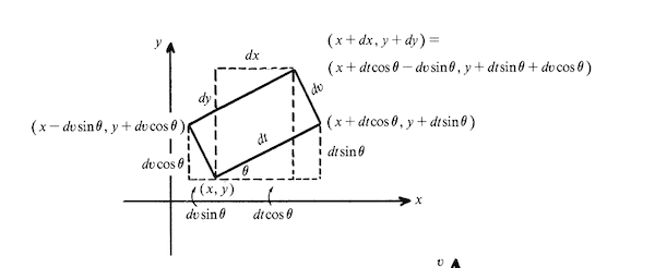
The figure, taken from Katz, shows the translation, and rotation that should preserve area on a differential scale.
However Euler knew \(dx = (\partial{g_1}/\partial{t}) dt + (\partial{g_1}/\partial{v}) dv\) and \(dy = (\partial{g_2}/{\partial{t}}) dt + (\partial{g_2}/\partial{v}) dv\). Just multiplying gives \(dx dy = m\sqrt{1-m^2} dt dt + (1-m^2) dv dt -m^2 dt dv -m\sqrt{1-m^2} dv dv\), a result that didn’t make sense physically as \(dt dt\) and \(dv dv\) have no meaning in integration and \(1 - m^2 - m^2\) is not \(1\) as expected. Euler, like Lagrange, used a formal trick to proceed, but the geometric insight that the incremental areas for a change of variable should be related and for this change of variable identical is correct.
The following illustrates the polar-coordinate transformation \(\langle x,y\rangle = G(r, \theta) = r \langle \cos\theta, \sin\theta\rangle\).
G(u, v) = u * [cos(v), sin(v)]

G(v) = G(v...)
J(v) = ForwardDiff.jacobian(G, v)  # [∇g1', ∇g2']

n = 6
us = range(0, 1, length=3n)     # radius
vs = range(0, 2pi, length=3n)   # angle

plot(unzip(G.(us', vs))..., legend = false, aspect_ratio=:equal)  # plots constant u lines
plot!(unzip(G.(us, vs'))...)                                      # plots constant v lines

pt = [us[n],vs[n]]


arrow!(G(pt), J(pt)*[1,0], color=:blue)
arrow!(G(pt), J(pt)*[0,1], color=:blue)
This graphic shows the image of the box \([0,1] \times [0, 2\pi]\) under the transformation. The plot commands draw lines for values of constant u or constant v. If \(G(u,v) = \langle g_1(u,v), g_2(u,v)\rangle\), then the Taylor expansion for \(g_i\) is \(g_i(u+du, v+dv) \approx g_i(u,v) + (\nabla{g_i})^T \cdot \langle du, dv \rangle\) and combining \(G(u+du, v+dv) \approx G(u,v) + J_G(u,v) \langle du, dv \rangle\). The vectors added above represent the images when \(u\) is constant (so \(du=0\)) and when \(v\) is constant (so \(dv=0\)). The two arrows define a parallelogram whose area gives the change of area undergone by the unit square under the transformation. The area is \(|\det(J_G)|\), the absolute value of the determinant of the Jacobian.
showG (generic function with 3 methods)The transformation to elliptical coordinates, \(G(u,v) = \langle \cosh(u)\cos(v), \sinh(u)\sin(v)\rangle\), may be viewed similarly:
The transformation \(G(u,v) = v \langle e^u, e^{-u} \rangle\) uses hyperbolic coordinates:
The transformation \(G(u,v) = \langle u^2-v^2, u\cdot v \rangle\) yields a partition of the plane:
The arrows are the images of the standard unit vectors. We see some transformations leave these orthogonal and some change the respective lengths. The area of the associated parallelogram can be found using the determinant of an accompanying matrix. For two dimensions, using the cross product formulation on the embedded vectors, the area is
\[ \| \det\left( \begin{bmatrix} \hat{i} & \hat{j} & \hat{k}\\ u_1 & u_2 & 0\\ v_1 & v_2 & 0 \end{bmatrix} \right) \| = \| \hat{k} \det\left( \begin{bmatrix} u_1 & u_2\\ v_1 & v_2 \end{bmatrix} \right) \| = | \det\left( \begin{bmatrix} u_1 & u_2\\ v_1 & v_2 \end{bmatrix} \right)|. \]
Using the fact that the two vectors involved are columns in the Jacobian of the transformation, this is just \(|\det(J_G)|\). For \(3\) dimensions, the determinant gives the volume of the 3-dimensional parallelepiped in the same manner. This holds for higher dimensions.
The absolute value of the determinant of the Jacobian is the multiplying factor that is seen in the change of variable formula for all dimensions:
For the one-dimensional case, there is no absolute value, but there the interval is reversed, producing “negative” area. This is not the case here, where \(S\) is parameterized to give positive volume.
NoteNote
The term “functional determinant” is found for the value \(\det(J_G)\), as is the notation \(\partial(x_1, x_2, \dots x_n)/\partial(u_1, u_2, \dots, u_n)\).
63.5.1 Two dimensional change of variables
Now we see several examples of two-dimensional transformations.
Polar integrals
We have seen how to compute area in polar coordinates through the formula \(A = \int (1/2) r^2(\theta) d\theta\). This formula can be derived as follows. Consider a region \(R\) parameterized in polar coordinates by \(r(\theta)\) for \(a \leq \theta \leq b\). The area of this region would be \(\iint_R 1dA\). Let \(G(r, \theta) = r \langle \cos\theta, \sin\theta\rangle\). Then
\[ J_G = \begin{bmatrix} \cos(\theta) & - r\sin(\theta)\\ \sin(\theta) & r\cos(\theta) \end{bmatrix}, \]
with determinant \(r\).
That is, for polar coordinates \(dx dy = r dr d\theta\) (\(r \geq 0\)).
So by the change of variable formula, we have:
\[ A = \iint_R 1 dx dy = \int_a^b \int_0^{r(\theta)} 1 r dr d\theta = \int_a^b \frac{r^2(\theta)}{2} d\theta. \]
The key is noting that the region, \(S\), described by \(\theta\) running from \(a\) to \(b\) and \(r\) running from \(0\) to \(r(\theta)\), maps onto \(R\) through the change of variables. As polar coordinates is just a renaming, this is clear to see.
Now consider finding the volume of a sphere using polar coordinates. We have, with \(\rho\) being the radius:
\[ V = 2 \iint_R \sqrt{\rho^2 - x^2 - y^2} dy dx, \]
where \(R\) is the disc of radius \(\rho\). Using polar coordinates, we have \(x^2 + y^2 = r^2\) and the expression becomes:
\[ V = 2 \int_0^{2\pi} \int_0^\rho \sqrt{\rho^2 - r^2} r dr d\theta = 2 \int_0^{2\pi} -(\rho^2 - r^2)^{3/2}\frac{1}{3} \mid_0^\rho d\theta = 2\int_0^{2\pi} \frac{\rho^3}{3}d\theta = \frac{4\pi\rho^3}{3}. \]
Linear transformations
Some transformations from \(2\)D computer graphics are represented in matrix notation:
\[ \begin{bmatrix} x\\ y \end{bmatrix} = \begin{bmatrix} a & b\\ c & d \end{bmatrix} \begin{bmatrix} u\\ v \end{bmatrix} , \]
or \(G(u,v) = \langle au+bv, cu+dv\rangle\). The Jacobian of this linear transformation is the matrix itself.
Some common transformations are:
- Stretching or \(G(u,v) = \langle ku, v \rangle\) or \(G(u,v) = \langle u, kv\rangle\) for some \(k >0\). The former stretching the \(x\) axis, the latter the \(y\). These have Jacobian determinant \(k\)
- Rotation. Let \(\theta\) be a clockwise rotation parameter, then \(G(u,v) = \langle\cos\theta u + \sin\theta v, -\sin\theta u + \cos\theta v\rangle\) will be the transform. The Jacobian is \(1\). This figure rotates by \(\pi/6\):
- Shearing. Let \(k > 0\) and \(G(u,v) = \langle u + kv, v \rangle\). This transformation is shear parallel to the \(x\) axis. (Use \(G(u,v) = \langle u, ku+v\rangle\) for the \(y\) axis). A shear has Jacobian \(1\).
k = 2
G(u, v) = [u + 2v, v]
showG(G)- Reflection If \(\vec{l} = \langle l_x, l_y \rangle\) with norm \(\|\vec{l}\|\). The reflection through the line in the direction of \(\vec{l}\) through the origin is defined, using a matrix, by:
\[ \frac{1}{\| \vec{l} \|^2} \begin{bmatrix} l_x^2 - l_y^2 & 2 l_x l_y\\ 2l_x l_y & l_y^2 - l_x^2 \end{bmatrix} \]
For some simple cases: \(\langle l_x, l_y \rangle = \langle 1, 1\rangle\), the diagonal, this is \(G(u,v) = (1/2) \langle 2v, 2u \rangle\); \(\langle l_x, l_y \rangle = \langle 0, 1\rangle\) (the \(y\)-axis) this is \(G(u,v) = \langle -u, v\rangle\).
- A translation by \(\langle a ,b \rangle\) would be given by \(G(u,v) = \langle u+a, v+b \rangle\) and would have Jacobian determinant \(1\).
As an example, consider the transformation of reflecting through the line \(x = 1/2\). Let \(\vec{ab} = \langle 1/2, 0\rangle\). This would be found by translating by \(-\vec{ab}\) then reflecting through the \(y\) axis, then translating by \(\vec{ab}\):
T(u, v, a, b) = [u+a, v+b]
G(u, v) = [-u, v]
@syms u v
a,b = 1//2, 0
x1, y1 = T(u,v, -a, -b)
x2, y2 = G(x1, y1)
x, y = T(x2, y2, a, b)
\(\left[\begin{smallmatrix}1 - u\\v\end{smallmatrix}\right]\)
Triangle
Consider the problem of integrating \(f(x,y)\) over the triangular region bounded by \(y=x\), \(y=0\), and \(x=1\). Such an integral may be computed through Fubini’s theorem through \(\int_0^1 \int_0^x f(x,y) dy dx\) or \(\int_0^1 \int_y^1 f(x,y) dx dy\), but if these can not be computed, and a numeric option is preferred, a transformation so that the integral is over a rectangle is preferred.
For this, the transformation \(x = u\), \(y=uv\) for \((u,v)\) in \([0,1] \times [0,1]\) is possible:
The determinant of the Jacobian is
\[ \det(J_G) = \det\left( \begin{bmatrix} 1 & 0\\ v & u \end{bmatrix} \right) = u. \]
So, \(\iint_R f(x,y) dA = \int_0^1\int_0^1 f(u, uv) u du dv\). Here we illustrate with a generic monomial:
@syms x y n::positive m::positive
monomial(x,y) = x^n*y^m
integrate(monomial(x,y), (y, 0, x), (x, 0, 1))
\(\frac{1}{\left(m + 1\right) \left(m + n + 2\right)}\)
And compare with:
@syms u v
integrate(monomial(u, u*v)*u, (u,0,1), (v,0,1))
\(\frac{1}{\left(m + 1\right) \left(m + n + 2\right)}\)
Composition of transformations
What about other triangles, say the triangle bounded by \(x=0\), \(y=0\) and \(y-x=1\)?
This can be seen as a reflection through the line \(x=1/2\) of the triangle above. If \(G_1\) represents the mapping from \(U [0,1]\times[0,1]\) into the triangle of the last problem, and \(G_2\) represents the reflection through the line \(x=1/2\), then the transformation \(G_2 \circ G_1\) will map the box \(U\) into the desired region. By the chain rule, we have:
\[ \begin{align*} \int_{(G_2\circ G_1)(U)} f dx &= \int_U (f\circ G_2 \circ G_1) |\det(J_{G_2 \circ G_1})| du \\ &= \int_U (f\circ G_2 \circ G_1) |\det(J_{G_2}(G_1(u)))||\det(J_{G_1}(u))| du. \end{align*} \]
(In Katz it is mentioned that Jacobi showed this in 1841.)
The flip through the \(x=1/2\) line was done above and is \(\langle u, v\rangle \rightarrow \langle 1-u, v\rangle\) which has Jacobian determinant \(-1\).
We compare now using and hcubature and our “Fubini” function:
G1(u,v) = [u, u*v]
G1(v) = G1(v...)
G2(u,v) = [1-u, v]
G2(v) = G2(v...)
f(x,y) = x^2*y^3
f(v) = f(v...)
A = ∬((y,x) -> f(x,y), (0, x -> 1 - x), (0, 1))
B = hcubature(v -> (f∘G2∘G1)(v) * v[1] * 1, (0,0), (1, 1))
A, B[1], A - B[1]
(0.0023809523809523807, 0.0023809523809509895, 1.3912482277333993e-15)Hyperbolic transformation
Consider the region, \(R\), bounded by \(y=0\), \(x=e^{-n}\), \(x=e^n\), and \(y=1/x\). An integral over this region may be computed with the help of the transform \(G(u,v) = v \langle e^u, e^{-u}\rangle\) which takes the box \([-n, n] \times [0,1]\) onto \(R\).
With this, we compute \(\iint_R x^2 y^3 dA\) using SymPy to compute the Jacobian:
@syms u v n
G(u,v) = v * [exp(u), exp(-u)]
Jac = G(u,v).jacobian([u,v])
f(x,y) = x^2 * y^3
f(v) = f(v...)
integrate(f(G(u,v)) * abs(det(Jac)), (u, -n, n), (v, 0, 1))
\(\frac{\left(2 e^{2 n} - 2\right) e^{- n}}{7}\)
This collection shows a summary of the above \(2\)D transformations:
63.5.2 Examples
Centroid:
The center of mass is a balancing point of a region with density \(\rho(x,y)\). In two dimensions it is a point \(\langle \bar{x}, \bar{y}\rangle\). These are found by the following formulas:
\[ A = \iint_R \rho(x,y) dA, \quad \bar{x} = \frac{1}{A} \iint_R x \rho(x,y) dA, \quad \bar{y} = \frac{1}{A} \iint_R y \rho(x,y) dA. \]
The \(x\) value can be seen in terms of Fubini by integrating in \(y\) first:
\[ \iint_R x \rho(x,y) dA = \int_{x=a}^b x (\int_{y=h(x)}^{g(x)} \rho(x,y) dy) dx. \]
The inner integral is the mass of a slice at a value along the \(x\) axis. The center of mass is formed then by the mass times the distance from the origin. The center of mass is a “balance” point, in the sense that \(\iint_R (x - \bar{x}) dA = 0\) and \(\iint_R (y-\bar{y})dA = 0\).
For example, the center of mass of the upper half unit disc will have a centroid with \(\bar{x} = 0\), by symmetry. We can see this by integrating in Cartesian coordinates, as follows
\[ \iint_R x dA = \int_{y=0}^1 \int_{x=-\sqrt{1-y^2}}^{\sqrt{1 - y^2}} x dx dy. \]
The inner integral is \(0\) as it an integral of an odd function over an interval symmetric about \(0\).
The value of \(\bar{y}\) is found using polar coordinate transformation from:
\[ \iint_R y dA = \int_{r=0}^1 \int_{\theta=0}^{\pi} (r\sin(\theta))r d\theta dr = \int_{r=0}^1 r^2 dr \int_{\theta=0}^{\pi}\sin(\theta) d\theta = \frac{1}{3} \cdot 2. \]
The third equals sign uses separability. The answer for \(\bar{y}\) is this value divided by the area, or \(4/(3\pi)\).
Example: Moment of inertia
The moment of inertia of a point mass about an axis is \(I = mr^2\) where \(m\) is the mass and \(r\) the distance to the axis. The moment of inertia of a body is the sum of the moment of inertia of each piece. If \(R\) is a region in the \(x\)-\(y\) plane with density \(\rho(x,y)\) and the axis is the \(y\) axis, then an approximate moment of inertia would be \(\sum (x_i)^2\rho(x_i, y_i)\Delta x_i \Delta y_i\) which would lead to \(I = \iint_R x^2\rho(x,y) dA\).
Let \(R\) be the half disc contained by \(x^2 + y^2 = 1\) and \(x \geq 0\). Let \(\rho(x,y) = xy^2\). Find the moment of inertia.
\[ R \]
is best described in polar coordinates, so we try to compute
\[ \int_0^1 \int_{-\pi/2}^{\pi/2} (r\cos(\theta))^2 (r\cos(\theta))(r\sin(\theta))^2 r d\theta dr. \]
That requires integrating \(\sin^2(\theta)\cos^3(\theta)\), a doable task, but best left to SymPy:
@syms r theta
x = r*cos(theta)
y = r*sin(theta)
rho(x,y) = x*y^2
integrate(x^2 * rho(x, y), (theta, -PI/2, PI/2), (r, 0, 1))
\(\frac{2}{45}\)
Example
(Strang) Find the moment of inertia about the \(y\) axis of the unit square tilted counter-clockwise an angle \(0 \leq \alpha \leq \pi/2\).
The counterclockwise rotation of the unit square is \(G(u,v) = \langle \cos(\alpha)u-\sin(\alpha)v, \sin(\alpha)u + \cos(\alpha) v\rangle\). This comes from the above formula for clockwise rotation using \(-\alpha\). This transformation has Jacobian determinant \(1\), as the area is not deformed. With this, we have
\[ \iint_R x^2 dA = \iint_{G(U)} (f\circ G)(u) |\det(J_G(u))| dU, \]
which is computed with:
@syms u v alpha
f(x,y) = x^2
G(u,v) = [cos(alpha)*u - sin(alpha)*v, sin(alpha)*u + cos(alpha)*v]
Jac = det(G(u,v).jacobian([u,v])) |> simplify
integrate(f(G(u,v)...) * Jac , (u,  0, 1), (v, 0, 1))
\(\frac{\sin^{2}{\left(\alpha \right)}}{3} - \frac{\sin{\left(\alpha \right)} \cos{\left(\alpha \right)}}{2} + \frac{\cos^{2}{\left(\alpha \right)}}{3}\)
Example
Let \(R\) be a ring with inner radius \(4\) and outer radius \(5\). Find its moment of inertia about the \(y\) axis.
The integral to compute is:
\[ \iint_R x^2 dA, \]
with domain that is easy to describe in polar coordinates:
@syms r theta
x = r*cos(theta)
integrate(x^2 * r, (r, 4, 5), (theta, 0, 2PI))
\(\frac{369 \pi}{4}\)
63.5.3 Three dimensional change of variables
The change of variables formula is no different between dimensions \(2\) and \(3\) (or higher), but the question of suitable transformation is more involved as the dimensions increase. We stick here to a few widely used ones.
Cylindrical coordinates
Polar coordinates describe the \(x\)-\(y\) plane in terms of a radius \(r\) and angle \(\theta\). Cylindrical coordinates describe the \(x-y-z\) plane in terms of \(r, \theta\), and \(z\). A transformation is:
\[ G(r,\theta, z) = \langle r\cos(\theta), r\sin(\theta), z\rangle. \]
This has Jacobian determinant \(r\), similar to polar coordinates.
Example
Returning to the volume of a cone above the \(x\)-\(y\) plane under \(z = a - b(x^2 + y^2)^{1/2}\). This yielded the integral in Cartesian coordinates:
\[ \int_{x=-r}^r \int_{y=-\sqrt{r^2 - x^2}}^{\sqrt{r^2-x^2}} \int_0^{a - b(x^2 + y^2)^{1/2}} 1 dz dy dx, \]
where \(r=a/b\). This is much simpler in Cylindrical coordinates, as the region is described by the rectangle in \((r, \theta)\): \([0, a/b] \times [0, 2\pi]\) and the \(z\) range is from \(0\) to \(a - b r\).
The volume then is:
\[ \int_{theta=0}^{2\pi} \int_{r=0}^{a/b} \int_{z=0}^{a - br} 1 r dz dr d\theta = 2\pi \int_{r=0}^{a/b} (a-br)r dr = \frac{\pi a^3}{3b^2}. \]
This is in agreement with \(\pi r^2 h/3\).
Find the centroid for the cone. First in the \(x\) direction, \(\iint_R x dV\) is found by:
@syms r theta z a b
f(x,y,z) = x
x = r*cos(theta)
y = r*sin(theta)
Jac = r
integrate(f(x,y,z) * Jac, (z, 0, a - b*r), (r, 0, a/b), (theta, 0, 2PI))
\(0\)
That this is \(0\) is no surprise. The same will be true for the \(y\) direction, as the figure is symmetric about the plane \(y=0\) and \(x=0\). However, the \(z\) direction is different:
@syms r theta z a b
f(x,y,z) = z
x = r*cos(theta)
y = r*sin(theta)
Jac = r
A = integrate(f(x,y,z) * Jac, (z, 0, a - b*r), (r, 0, a/b), (theta, 0, 2PI))
B = integrate(1 * Jac, (z, 0, a - b*r), (r, 0, a/b), (theta, 0, 2PI))
A, B, A/B
(pi*a^4/(12*b^2), pi*a^3/(3*b^2), a/4)The answer depends on the height through \(a\), but not the size of the base, parameterized by \(b\). To finish, the centroid is \(\langle 0, 0, a/4\rangle\).
Example
A sphere of radius \(2\) is intersected by a cylinder of radius \(1\) along the \(z\) axis. Find the volume of the intersection.
We have \(x^2 + y^2 + z^2 = 4\) or \(z^2 = 4 - r^2\) in cylindrical coordinates. The integral then is:
@syms r::real theta::real z::real
integrate(1 * r, (z, -sqrt(4-r^2), sqrt(4-r^2)), (r, 0, 1), (theta, 0, 2PI))
\(2 \pi \left(\frac{16}{3} - 2 \sqrt{3}\right)\)
If instead of a fixed radius of \(1\) we use \(0 \leq a \leq 2\) we have:
@syms a r theta
integrate(1 * r, (z, -sqrt(4-r^2), sqrt(4-r^2)), (r, 0, a), (theta,0, 2PI))
\(2 \pi \left(\frac{2 a^{2} \sqrt{4 - a^{2}}}{3} - \frac{8 \sqrt{4 - a^{2}}}{3} + \frac{16}{3}\right)\)
Spherical integrals
Spherical coordinates describe a point in space by a radius from the origin, \(r\) or \(\rho\); an azimuthal angle \(\theta\) in \([0, 2\pi]\) and an inclination angle \(\phi\) (also called polar angle) in \([0, \pi]\). The \(z\) axis is the direction of the zenith and gives a reference line to define the inclination angle. The \(x\)-\(y\) plane is the reference plane, with the \(x\) axis giving a reference direction for the azimuth measurement.
The exact formula to relate \((\rho, \theta, \phi)\) to \((x,y,z)\) is given by
\[ G(\rho, \theta, \phi) = \rho \langle \sin(\phi)\cos(\theta), \sin(\phi)\sin(\theta), \cos(\phi) \rangle. \]
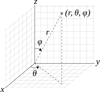
The Jacobian can be computed to be \(\rho^2\sin(\phi)\).
@syms ρ θ ϕ
G(ρ, θ, ϕ) = ρ * [sin(ϕ)*cos(θ), sin(ϕ)*sin(θ), cos(ϕ)]
det(G(ρ, θ, ϕ).jacobian([ρ, θ, ϕ])) |> simplify |> abs
\(\left|{ρ^{2} \sin{\left(ϕ \right)}}\right|\)
Example
Computing the volume of a sphere is a challenge (for SymPy) in Cartesian coordinates, but a breeze in spherical coordinates. Using \(r^2\sin(\phi)\) as the multiplying factor, the volume is simply:
\[ \int_{\theta=0}^{2\pi} \int_{\phi=0}^{\pi} \int_{r=0}^R 1 \cdot r^2 \sin(\phi) dr d\phi d\theta = \int_{\theta=0}^{2\pi} d\theta \int_{\phi=0}^{\pi} \sin(\phi)d\phi \int_{r=0}^R r^2 dr = (2\pi)(2)\frac{R^3}{3} = \frac{4\pi R^3}{3}. \]
Example
Compute the volume of the ellipsoid, \(R\), described by \((x/a)^2 + (y/b)^2 + (z/c)^2 \leq 1\).
We first change variables via \(G(u,v,w) = \langle ua, vb, wc \rangle\). This maps the unit sphere, \(S\), given by \(u^2 + v^2 + w^2 \leq 1\) into the ellipsoid. Then
\[ \iint_R 1 dV = \iint_S 1 |\det(J_G)| dU \]
But the Jacobian is a constant:
@syms u v w a b c
G(u,v,w) = [u*a, v*b, w*c]
det(G(u,v,w).jacobian([u,v,w]))
\(a b c\)
So the answer is \(abc V(S) = 4\pi abc/3\)
63.6 Questions
Question
Suppose \(f(x,y) = f_1(x)f_2(y)\) and \(R = [a_1, b_1] \times [a_2,b_2]\) is a rectangular region. Is this true?
\[ \iint_R f dA = (\int_{a_1}^{b_1} f_1(x) dx) \cdot (\int_{a_2}^{b_2} f_2(y) dy). \]
Question
Which integrals of the following are \(0\) by symmetry? Let \(R\) be the unit disc.
\[ a = \iint_R x dA, \quad b = \iint_R (x^2 + y^2) dA, \quad c = \iint_R xy dA \]
Question
Let \(R\) be the unit disc. Which integrals can be found from common geometric formulas (e.g., known formulas for the sphere, cone, pyramid, ellipse, …)
\[ a = \iint_R (1 - (x^2+y^2)) dA, \quad b = \iint_R (1 - \sqrt{x^2 + y^2}) dA, \quad c = \iint_R (1 - (x^2 + y^2)^2 dA \]
Question
Let the region \(R\) be described by: in the first quadrant and bounded by \(x^3 + y^3 = 1\). What integral below will not find the area of \(R\)?
Question
Let \(R\) be a triangular region with vertices \((0,0), (2,0), (1, b)\) where \(b \geq 0\). What integral below computes the area of \(R\)?
Question
Let \(f(x) \geq 0\) be an integrable function. The area under \(f(x)\) over \([a,b]\), \(\int_a^b f(x) dx\), is equivalent to?
Question
The region \(R\) contained within \(|x| + |y| = 1\) is square, but not rectangular (in the sense of integration). What transformation of \(S = [-1/2,1/2] \times [-1/2,1/2]\) will have \(G(S) = R\)?
Question
Let \(G(u,v) = \langle \cosh(u)\cos(v), \sinh(u)\sin(v) \rangle\). Using ForwardDiff find the determinant of the Jacobian at \([1,2]\).
Question
Let \(G(u, v) = \langle \cosh(u)\cos(v), \sinh(u)\sin(v) \rangle\). Compute the determinant of the Jacobian symbolically:
Question
Compute the determinant of the Jacobian of the composition of a clockwise rotation by \(\theta\), a reflection through the \(x\) axis, and then a translation by \(\langle a,b\rangle\), using the fact that the Jacobian determinant of compositions can be written as product of determinants of the individual Jacobians.
Question
A wedge, \(R\), is specified by \(0 \leq r \leq a\), \(0 \leq \theta \leq b\).
@syms r theta a b
x = r*cos(theta)
y = r*sin(theta)
A = integrate(r, (r, 0, a), (theta, 0, b))
B = integrate(x * r, (r, 0, a), (theta, 0, b))
C = integrate(y * r, (r, 0, a), (theta, 0, b))
\(- \frac{a^{3} \cos{\left(b \right)}}{3} + \frac{a^{3}}{3}\)
What does A compute?
What does \(B/A\) compute?
Question
According to Katz in 1899 Cartan formalized the subject of differential forms (elements such as \(dx\) or \(du\)). Using the rules \(dtdt = 0 = dvdv\) and \(dv dt = - dt dv\), what is the product of \(dx=mdt + dv\sqrt{1-m^2}\) and \(dy=dt\sqrt{1-m^2}-mdv\)?