59  Functions \(R^n \rightarrow R^m\)

This section uses these add-on packages:

using CalculusWithJulia
using Plots
plotly()
using SymPy
using ForwardDiff
using LinearAlgebra

For a scalar function \(f: R^n \rightarrow R\), the gradient of \(f\), \(\nabla{f}\), is a function from \(R^n \rightarrow R^n\). Specializing to \(n=2\), a function that for each point, \((x,y)\), assigns a vector \(\vec{v}\). This is an example of vector field. More generally, we could have a function \(f: R^n \rightarrow R^m\), of which we have discussed many already:

Mapping	Name	Visualize with	Notation
\(f: R\rightarrow R\)	univariate	familiar graph of function	\(f\)
\(f: R\rightarrow R^m\)	vector-valued	space curve when n=2 or 3	\(\vec{r}\), \(\vec{N}\)
\(f: R^n\rightarrow R\)	scalar	a surface when n=2	\(f\)
\(F: R^n\rightarrow R^n\)	vector field	a vector field when n=2, 3	\(F\)
\(F: R^n\rightarrow R^m\)	multivariable	n=2,m=3 describes a surface	\(F\), \(\Phi\)

After an example where the use of a multivariable function is of necessity, we discuss differentiation in general for a multivariable functions.

59.1 Vector fields

We have seen that the gradient of a scalar function, \(f:R^2 \rightarrow R\), takes a point in \(R^2\) and associates a vector in \(R^2\). As such \(\nabla{f}:R^2 \rightarrow R^2\) is a vector field. A vector field is a vector-valued function from \(R^n \rightarrow R^n\) for \(n \geq 2\).

An input/output pair can be visualized by identifying the input values as a point, and the output as a vector visualized by anchoring the vector at the point. A vector field is a sampling of such pairs, usually taken over some ordered grid. The details, as previously mentioned, are in the vectorfieldplot function of CalculusWithJulia.

F(u,v) = [-v, u]
vectorfieldplot(F, xlim=(-5,5), ylim=(-5,5), nx=10, ny=10)

The optional arguments nx=10 and ny=10 determine the number of points on the grid that a vector will be plotted. These vectors are scaled to not overlap.

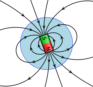
Vector field plots are useful for visualizing velocity fields, where a velocity vector is associated to each point; or streamlines, curves whose tangents are follow the velocity vector of a flow. Vector fields are used in physics to model the electric field and the magnetic field. These are used to describe forces on objects within the field.

The three dimensional vector field is one way to illustrate a vector field, but there is an alternate using field lines. Like Euler’s method, imagine starting at some point, \(\vec{r}\) in \(R^3\). The field at that point is a vector indicating a direction of motion. Follow that vector for some infinitesimal amount, \(d\vec{r}\). From here repeat. The field curve would satisfy \(\vec{r}'(t) = F(\vec{r}(t))\). Field curves only show direction, to indicate magnitude at a point, the convention is to use denser lines when the field is stronger.

Illustration of the magnetic field of the earth using field lines to indicate the field. From Wikipedia.

---

Vector fields are also useful for other purposes, such as transformations, examples of which are a rotation or the conversion from polar to rectangular coordinates.

For transformations, a useful visualization is to plot curves where one variables is fixed. Consider the transformation from polar coordinates to cartesian coordinates \(F(r, \theta) = r \langle\cos(\theta),\sin(\theta)\rangle\). The following plot will show in blue fixed values of \(r\) (circles) and in red fixed values of \(\theta\) (rays).

F(r,theta) = r*[cos(theta), sin(theta)]
F(v) = F(v...)

rs = range(0, 2, length=5)
thetas = range(0, pi/2, length=9)

plot(legend=false, aspect_ratio=:equal)
plot!(unzip(F.(rs, thetas'))..., color=:red)
plot!(unzip(F.(rs', thetas))..., color=:blue)

pt = [1, pi/4]
J = ForwardDiff.jacobian(F, pt)
arrow!(F(pt...), J[:,1], linewidth=5, color=:red)
arrow!(F(pt...), J[:,2], linewidth=5, color=:blue)

pt = [0.5, pi/8]
J = ForwardDiff.jacobian(F, pt)
arrow!(F(pt...), J[:,1], linewidth=5, color=:red)
arrow!(F(pt...), J[:,2], linewidth=5, color=:blue)

Figure 59.1: Plot of a vector field from \(R^2 \rightarrow R^2\) illustrated by drawing curves with fixed \(r\) and \(\theta\). The partial derivatives are added as layers.

To the plot, we added the partial derivatives with respect to \(r\) (in red) and with respect to \(\theta\) (in blue). These are found with the soon-to-be discussed Jacobian. From the graph, you can see that these vectors are tangent vectors to the drawn curves.

The curves form a non-rectangular grid. Were the cells exactly parallelograms, the area would be computed taking into account the length of the vectors and the angle between them—the same values that come out of a cross product.

59.2 Parametrically defined surfaces

For a one-dimensional curve we have several descriptions. For example, as the graph of a function \(y=f(x)\); as a parametrically defined curve \(\vec{r}(t) = \langle x(t), y(t)\rangle\); or as a level curve of a scalar function \(f(x,y) = c\).

For two-dimensional surfaces in three dimensions, we have discussed describing these in terms of a function \(z = f(x,y)\) and as level curves of scalar functions: \(c = f(x,y,z)\). They can also be described parametrically.

We pick a familiar case, to make this concrete: the unit sphere in \(R^3\). We have

• It is described by two functions through \(f(x,y) = \pm \sqrt{1 - (x^2 + y^2)}\).
• It is described by \(f(x,y,z) = 1\), where \(f(x,y,z) = x^2 + y^2 + z^2\).
• It can be described in terms of spherical coordinates:

\[ \Phi(\theta, \phi) = \langle \sin(\phi)\cos(\theta), \sin(\phi)\sin(\theta), \cos(\phi) \rangle, \]

with \(\theta\) the azimuthal angle and \(\phi\) the polar angle (measured down from the \(z\) axis).

The function \(\Phi\) takes \(R^2\) into \(R^3\), so is a multivariable function.

When a surface is described by a function, \(z=f(x,y)\), then the gradient points (in the \(x-y\) plane) in the direction of greatest increase of \(f\). The vector \(\langle -f_x, -f_y, 1\rangle\) is a normal.

When a surface is described as a level curve, \(f(x,y,z) = c\), then the gradient is normal to the surface.

When a surface is described parametrically, there is no “gradient.” The partial derivatives are of interest, e.g., \(\partial{F}/\partial{\theta}\) and \(\partial{F}/\partial{\phi}\), vectors defined componentwise. These will be lie in the tangent plane of the surface, as they can be viewed as tangent vectors for parametrically defined curves on the surface. Their cross product will be normal to the surface. The magnitude of the cross product, which reflects the angle between the two partial derivatives, will be informative as to the surface area.

59.2.1 Plotting parameterized surfaces in Julia

Consider the parametrically described surface above. How would it be plotted? Using the Plots package, the process is quite similar to how a surface described by a function is plotted, but the \(z\) values must be computed prior to plotting.

Here we define the parameterization using functions to represent each component:

X(theta,phi) = sin(phi) * cos(theta)
Y(theta,phi) = sin(phi) * sin(theta)
Z(theta,phi) = cos(phi)

Z (generic function with 1 method)

Then:

thetas = range(0, stop=pi/2, length=50)
phis   = range(0, stop=pi,   length=50)

xs = [X(theta, phi) for theta in thetas, phi in phis]
ys = [Y(theta, phi) for theta in thetas, phi in phis]
zs = [Z(theta, phi) for theta in thetas, phi in phis]

surface(xs, ys, zs)  ## see note

Note

PyPlot can be used directly to make these surface plots: import PyPlot; PyPlot.plot_surface(xs,ys,zs).

Instead of the comprehension, broadcasting can be used

surface(X.(thetas, phis'), Y.(thetas, phis'), Z.(thetas, phis'))

If the parameterization is presented as a function, broadcasting can be used to succinctly plot

Phi(theta, phi) = [X(theta, phi), Y(theta, phi), Z(theta, phi)]

surface(unzip(Phi.(thetas, phis'))...)

The partial derivatives of each component, \(\partial{\Phi}/\partial{\theta}\) and \(\partial{\Phi}/\partial{\phi}\), can be computed directly:

\[ \begin{align*} \partial{\Phi}/\partial{\theta} &= \langle -\sin(\phi)\sin(\theta), \sin(\phi)\cos(\theta),0 \rangle,\\ \partial{\Phi}/\partial{\phi} &= \langle \cos(\phi)\cos(\theta), \cos(\phi)\sin(\theta), -\sin(\phi) \rangle. \end{align*} \]

Using SymPy, we can compute through:

@syms theta phi
out = [diff.(Phi(theta, phi), theta) diff.(Phi(theta, phi), phi)]

\(\left[\begin{smallmatrix}- \sin{\left(\phi \right)} \sin{\left(\theta \right)} & \cos{\left(\phi \right)} \cos{\left(\theta \right)}\\\sin{\left(\phi \right)} \cos{\left(\theta \right)} & \sin{\left(\theta \right)} \cos{\left(\phi \right)}\\0 & - \sin{\left(\phi \right)}\end{smallmatrix}\right]\)

At the point \((\theta, \phi) = (\pi/12, \pi/6)\) this evaluates to the following.

subs.(out, theta=> PI/12, phi=>PI/6) .|> N

3×2 Matrix{Real}:
 -0.12941     0.836516
  0.482963    0.224144
  0         -1//2

We found numeric values, so that we can compare to the numerically identical values computed by the jacobian function from ForwardDiff:

pt = [pi/12, pi/6]
out₁ = ForwardDiff.jacobian(v -> Phi(v...), pt)

3×2 Matrix{Float64}:
 -0.12941    0.836516
  0.482963   0.224144
 -0.0       -0.5

What this function computes exactly will be described next, but here we visualize the partial derivatives and see they lie in the tangent plane at the point:

us, vs = range(0, pi/2, length=25), range(0, pi, length=25)
xs, ys, zs = unzip(Phi.(us, vs'))
surface(xs, ys, zs, legend=false)
arrow!(Phi(pt...), out₁[:,1], linewidth=3)
arrow!(Phi(pt...), out₁[:,2], linewidth=3)

Example: A detour into plotting

The presentation of a 3D figure in a 2D format requires the use of linear perspective. The Plots package adds lighting effects, to nicely render a surface, as seen.

In this example, we see some of the mathematics behind how drawing a surface can be done more primitively to showcase some facts about vectors. We follow a few techniques learned from Angenent (2012).

For our purposes we wish to mathematically project a figure onto a 2D plane.

The plane here is described by a view point in 3D space, \(\vec{v}\). Taking this as one vector in an orthogonal coordinate system, the other two can be easily produced, the first by switching two coordinates, as would be done in 2D; the second through the cross product:

function projection_plane(v)
    vx, vy, vz = v
    a = [-vy, vx, 0] # v ⋅ a = 0
    b = v × a        # so v ⋅ b = 0
    return (a/norm(a), b/norm(b))
end

projection_plane (generic function with 1 method)

Using these two unit vectors to describe the plane, the projection of a point onto the plane is simply found by taking dot products:

function project(x, v)
    â, b̂ = projection_plane(v)
    (x ⋅ â, x ⋅ b̂)    # (x ⋅ â) â + (x ⋅ b̂) b̂
end

project (generic function with 1 method)

Let’s see this in action by plotting a surface of revolution given by

radius(t) = 1 / (1 + exp(t))
t₀, tₙ = 0, 3
surf(t, θ) = [t, radius(t)*cos(θ), radius(t)*sin(θ)]

surf (generic function with 1 method)

We begin by fixing a view point and plotting the projected axes. We do the latter with a function for re-use.

v = [2, -2, 1]
function plot_axes()
    empty_style = (xaxis = ([], false),
                   yaxis = ([], false),
                   legend=false)

    plt = plot(; empty_style...)

    axis_values = [[(0,0,0), (3.5,0,0)],               # x axis
                   [(0,0,0), (0, 2.0 * radius(0), 0)], # yaxis
                   [(0,0,0), (0, 0, 1.5 * radius(0))]] # z axis

    for (ps, ax) ∈ zip(axis_values, ("x", "y", "z"))
        p0, p1 = ps
        a, b = project(p0, v), project(p1, v)
        annotate!([(b...,text(ax, :bottom))])
        plot!([a, b]; arrow=true, head=:tip, line=(:gray, 1)) # gr() allows arrows
    end

    plt
end

plt = plot_axes()

We are using the vector of tuples interface (representing points) to specify the curve to draw.

Now we add on some curves for fixed \(t\) and then fixed \(\theta\) utilizing the fact that project returns a tuple of \(x\)—\(y\) values to display.

for t in range(t₀, tₙ, 20)
    curve = [project(surf(t, θ), v) for θ in range(0, 2pi, 100)]
    plot!(curve; line=(:black, 1))
end
for θ in range(0, 2pi, 60)
    curve = [project(surf(t, θ), v) for t in range(t₀, tₙ, 20)]
    plot!(curve; line=(:black, 1))
end
plt

The graphic is a little busy!

Let’s focus on the cells layering the surface. These have equal size in the \(t \times \theta\) range, but unequal area on the screen. Where they parallellograms, the area could be found by taking the 2-dimensional cross product of the two partial derivatives, resulting in a formula like: \(a_x b_y - a_y b_x\). When we discuss integrals related to such figures, this amount of area will be characterized by a computation involving the determinant of the upcoming Jacobian function.

We make a function to close over the viewpoint vector that can be passed to ForwardDiff, as it will return a vector and not a tuple.

function psurf(v)
    (t,θ) -> begin
        v1, v2 = project(surf(t, θ), v)
        [v1, v2] # or call collect to make a tuple into a vector
    end
end

psurf (generic function with 1 method)

The function returned by psurf is from \(R^2 \rightarrow R^2\). With such a function, the computation of this approximate area becomes:

function detJ(F, t, θ)
    ∂θ = ForwardDiff.derivative(θ -> F(t, θ), θ)
    ∂t = ForwardDiff.derivative(t -> F(t, θ), t)
    (ax, ay), (bx, by) = ∂θ, ∂t
    ax * by - ay * bx
end

detJ (generic function with 1 method)

For our purposes, we are interested in the sign of the returned value. Plotting, we can see that some “area” is positive, some “negative”:

t = 1
G = psurf(v)
plot(θ -> detJ(G, t, θ), 0, 2pi)

With this parameterization and viewpoint, the positive area for the surface is when the normal vector points towards the viewing point. In the following, we only plot such values:

plt = plot_axes()

function I(F, t, θ)
    x, y = F(t, θ)
    detJ(F, t, θ) >= 0 ? (x, y) : (x, NaN) # use NaN for y value
end

for t in range(t₀, tₙ, 20)
    curve = [I(G, t, θ) for θ in range(0, 2pi, 100)]
    plot!(curve; line=(:gray, 1))
end

for θ in range(0, 2pi, 60)
    curve = [I(G, t, θ) for t in range(t₀, tₙ, 20)]
    plot!(curve; line=(:gray, 1))
end

plt

The values for which detJ is zero form the visible boundary of the object. We can plot just those to get an even less busy view. We identify them by finding the value of \(\theta\) in \([0,\pi]\) and \([\pi,2\pi]\) that makes the detJ function zero:

fold(F, t, θmin, θmax) = find_zero(θ -> detJ(F, t, θ), (θmin, θmax))

ts = range(t₀, tₙ, 100)
back_edge = fold.(G, ts, 0, pi)
front_edge = fold.(G, ts, pi, 2pi)

plt = plot_axes()
plot!(project.(surf.(ts, back_edge), (v,)); line=(:black, 1))
plot!(project.(surf.(ts, front_edge), (v,)); line=(:black, 1))

Adding caps makes the graphic stand out. The caps are just discs (fixed values of \(t\)) which are filled in with gray using a transparency so that the axes aren’t masked.

θs = range(0, 2pi, 100)
S = Shape(project.(surf.(t₀, θs), (v,)))
plot!(S; fill=(:gray, 0.33))

S = Shape(project.(surf.(tₙ, θs), (v,)))
plot!(S; fill=(:gray, 0.33))

Finally, we introduce some shading using the same technique but assuming the light comes from a different position.

lightpt = [2, -2, 5] # from further above
H = psurf(lightpt)
light_edge = fold.(H, ts, pi, 2pi);

Angles between the light edge and the front edge would be in shadow. We indicate this by drawing lines for fixed \(t\) values. As denser lines indicate more shadow, we feather how these are drawn:

for (i, (t, top, bottom)) in enumerate(zip(ts, light_edge, front_edge))
    λ = iseven(i) ? 1.0 : 0.8
    top = bottom + λ*(top - bottom)
    curve = [project(surf(t, θ), v) for θ in range(bottom, top, 20)]
    plot!(curve, line=(:black, 1))
end
plt

We can compare to the graph produced by surface for the same function:

ts = range(t₀, tₙ, 50)
θs = range(0, 2pi, 100)
surface(unzip(surf.(ts, θs'))...; legend=false)

59.3 The total derivative

Informally, the total derivative at \(a\) is the best linear approximation of the value of a function, \(F\), near \(a\) with respect to its arguments. If it exists, denote it \(dF_a\).

For a function \(F: R^n \rightarrow R^m\) we have the total derivative at \(\vec{a}\) (a point or vector in \(R^n\)) is a matrix \(J\) (a linear transformation) taking vectors in \(R^n\) and returning, under multiplication, vectors in \(R^m\) (this matrix will be \(m \times n\)), such that for some neighborhood of \(\vec{a}\), we have:

\[ \lim_{\vec{x} \rightarrow \vec{a}} \frac{\|F(\vec{x}) - F(\vec{a}) - J\cdot(\vec{x}-\vec{a})\|}{\|\vec{x} - \vec{a}\|} = \vec{0}. \]

(That is \(\|F(\vec{x}) - F(\vec{a}) - J\cdot(\vec{x}-\vec{a})\|=\mathcal{o}(\|\vec{x}-\vec{a}\|)\).)

If for some \(J\) the above holds, the function \(F\) is said to be totally differentiable, and the matrix \(J =J_F=dF_a\) is the total derivative.

For a multivariable function \(F:R^n \rightarrow R^m\), we may express the function in vector-valued form \(F(\vec{x}) = \langle f_1(\vec{x}), f_2(\vec{x}),\dots,f_m(\vec{x})\rangle\), each component a scalar function. Then, if the total derivative exists, it can be expressed by the Jacobian:

\[ J = \begin{bmatrix} \frac{\partial f_1}{\partial x_1} &\quad \frac{\partial f_1}{\partial x_2} &\dots&\quad\frac{\partial f_1}{\partial x_n}\\ \frac{\partial f_2}{\partial x_1} &\quad \frac{\partial f_2}{\partial x_2} &\dots&\quad\frac{\partial f_2}{\partial x_n}\\ &&\vdots&\\ \frac{\partial f_m}{\partial x_1} &\quad \frac{\partial f_m}{\partial x_2} &\dots&\quad\frac{\partial f_m}{\partial x_n} \end{bmatrix}. \]

This may also be viewed as:

\[ J = \begin{bmatrix} &\nabla{f_1}'\\ &\nabla{f_2}'\\ &\quad\vdots\\ &\nabla{f_m}' \end{bmatrix} = \left[ \frac{\partial{F}}{\partial{x_1}}\quad \frac{\partial{F}}{\partial{x_2}} \cdots \frac{\partial{F}}{\partial{x_n}} \right]. \]

The latter representing a matrix of \(m\) row vectors, each with \(n\) components or as a matrix of \(n\) column vectors, each with \(m\) components.

---

After specializing the total derivative to the cases already discussed, we have:

• Univariate functions. Here \(f'(t)\) is also univariate. Identifying \(J\) with the \(1 \times 1\) matrix with component \(f'(t)\), then the total derivative is just a restatement of the derivative existing.
• Vector-valued functions \(\vec{f}(t) = \langle f_1(t), f_2(t), \dots, f_m(t) \rangle\), each component univariate. Then the derivative, \(\vec{f}'(t) = \langle \frac{df_1}{dt}, \frac{df_2}{dt}, \dots, \frac{df_m}{dt} \rangle\). The total derivative in this case, is a \(m \times 1\) vector of partial derivatives, and since there is only \(1\) variable, would be written without partials. So the two agree.
• Scalar functions \(f(\vec{x}) = a\) of type \(R^n \rightarrow R\). The

definition of differentiability for \(f\) involved existence of the partial derivatives and moreover, the fact that a limit like the above held with \(\nabla{f}(C) \cdot \vec{h}\) in place of \(J\cdot(\vec{x}-\vec{a})\). Here \(\vec{h}\) and \(\vec{x}-\vec{a}\) are vectors in \(R^n\). Were the dot product in \(\nabla{f}(C) \cdot \vec{h}\) expressed in matrix multiplication we would have for this case a \(1 \times n\) matrix of the correct form:

\[ J = [\nabla{f}']. \]

• For \(f:R^2 \rightarrow R\), the Hessian matrix, was the matrix of \(2\)nd partial derivatives. This may be viewed as the total derivative of the the gradient function, \(\nabla{f}\):

\[ \text{Hessian} = \begin{bmatrix} \frac{\partial^2 f}{\partial x^2} &\quad \frac{\partial^2 f}{\partial x \partial y}\\ \frac{\partial^2 f}{\partial y \partial x} &\quad \frac{\partial^2 f}{\partial y \partial y} \end{bmatrix} \]

This is equivalent to:

\[ \begin{bmatrix} \frac{\partial \frac{\partial f}{\partial x}}{\partial x} &\quad \frac{\partial \frac{\partial f}{\partial x}}{\partial y}\\ \frac{\partial \frac{\partial f}{\partial y}}{\partial x} &\quad \frac{\partial \frac{\partial f}{\partial y}}{\partial y}\\ \end{bmatrix} . \]

As such, the total derivative is a generalization of what we have previously discussed.

59.4 The chain rule

If \(G:R^k \rightarrow R^n\) and \(F:R^n \rightarrow R^m\), then the composition \(F\circ G\) takes \(R^k \rightarrow R^m.\) If all three functions are totally differentiable, then a chain rule will hold (total derivative of \(F\circ G\) at point \(a\)):

\[ d(F\circ G)_a = dF_{G(a)} \cdot dG_a \]

If correct, this has the same formulation as the chain rule for the univariate case: derivative of outer at the inner times the derivative of the inner.

First we check that the dimensions are correct: We have \(dF_{G(a)}\) (the total derivative of \(F\) at the point \(G(a)\)) is an \(m \times n\) matrix and \(dG_a\) (the total derivative of \(G\) at the point \(a\)) is a \(n \times k\) matrix. The product of a \(m \times n\) matrix with a \(n \times k\) matrix is defined, and is a \(m \times k\) matrix, as is \(d(F \circ G)_a\).

The proof that the formula is correct uses the definition of totally differentiable written as

\[ F(b + \vec{h}) - F(b) - dF_b\cdot \vec{h} = \epsilon(\vec{h}) \vec{h}, \]

where \(\epsilon(h) \rightarrow \vec{0}\) as \(h \rightarrow \vec{0}\).

We have, using this for both \(F\) and \(G\):

\[ \begin{align*} F(G(a + \vec{h})) - F(G(a)) &= F(G(a) + (dG_a \cdot \vec{h} + \epsilon_G \vec{h})) - F(G(a))\\ &= F(G(a)) + dF_{G(a)} \cdot (dG_a \cdot \vec{h} + \epsilon_G \vec{h}) \\ &+ \quad\epsilon_F (dG_a \cdot \vec{h} + \epsilon_G \vec{h}) - F(G(a))\\ &= dF_{G(a)} \cdot (dG_a \cdot \vec{h}) + dF_{G(a)} \cdot (\epsilon_G \vec{h}) + \epsilon_F (dG_a \cdot \vec{h}) + (\epsilon_F \cdot \epsilon_G\vec{h}) \end{align*} \]

The last line uses the linearity of \(dF\) to isolate \(dF_{G(a)} \cdot (dG_a \cdot \vec{h})\). Factoring out \(\vec{h}\) and taking norms gives:

\[ \begin{align*} \frac{\| F(G(a+\vec{h})) - F(G(a)) - dF_{G(a)}dG_a \cdot \vec{h} \|}{\| \vec{h} \|} &= \frac{\| dF_{G(a)}\cdot(\epsilon_G\vec{h}) + \epsilon_F (dG_a\cdot \vec{h}) + (\epsilon_F\cdot\epsilon_G\vec{h}) \|}{\| \vec{h} \|} \\ &\leq \| dF_{G(a)}\cdot\epsilon_G + \epsilon_F (dG_a) + \epsilon_F\cdot\epsilon_G \|\frac{\|\vec{h}\|}{\| \vec{h} \|}\\ &\rightarrow 0. \end{align*} \]

59.4.1 Examples

Our main use of the total derivative will be the change of variables in integration.

Example: polar coordinates

A point \((a,b)\) in the plane can be described in polar coordinates by a radius \(r\) and polar angle \(\theta\). We can express this formally by \(F:(a,b) \rightarrow (r, \theta)\) with

\[ r(a,b) = \sqrt{a^2 + b^2}, \quad \theta(a,b) = \tan^{-1}(b/a), \]

the latter assuming the point is in quadrant I or IV (though atan(y,x) will properly handle the other quadrants). The Jacobian of this transformation may be found with

@syms a::real b::real

rⱼ = sqrt(a^2 + b^2)
θⱼ = atan(b/a)

Jac = Sym[diff.(rⱼ, [a,b])';        # [∇f_1'; ∇f_2']
          diff.(θⱼ, [a,b])']

simplify.(Jac)

\(\left[\begin{smallmatrix}a \overline{\frac{1}{\sqrt{a^{2} + b^{2}}}} & b \overline{\frac{1}{\sqrt{a^{2} + b^{2}}}}\\- \frac{b}{a^{2} + b^{2}} & \frac{a}{a^{2} + b^{2}}\end{smallmatrix}\right]\)

SymPy array objects have a jacobian method to make this easier to do. The calling style is Python-like, using object.method(...):

[rⱼ, θⱼ].jacobian([a, b])

\(\left[\begin{smallmatrix}\frac{a}{\sqrt{a^{2} + b^{2}}} & \frac{b}{\sqrt{a^{2} + b^{2}}}\\- \frac{b}{a^{2} \left(1 + \frac{b^{2}}{a^{2}}\right)} & \frac{1}{a \left(1 + \frac{b^{2}}{a^{2}}\right)}\end{smallmatrix}\right]\)

The determinant, of geometric interest, will be

det(Jac) |> simplify

\(\overline{\frac{1}{\sqrt{a^{2} + b^{2}}}}\)

The determinant is of interest, as the linear mapping represented by the Jacobian changes the area of the associated coordinate vectors. The determinant describes how this area changes, as a multiplying factor.

Example Spherical Coordinates

In \(3\) dimensions a point can be described by (among other ways):

• Cartesian coordinates: three coordinates relative to the \(x\), \(y\), and \(z\) axes as \((a,b,c)\).
• Spherical coordinates: a radius, \(r\), an azimuthal angle \(\theta\), and a polar angle

\[ \phi \]

measured down from the \(z\) axes. (We use the mathematics naming convention, the physics one has \(\phi\) and \(\theta\) reversed.)

• Cylindrical coordinates: a radius, \(r\), a polar angle \(\theta\), and height \(z\).

Some mappings are:

Cartesian (x,y,z)	Spherical (\(r\), \(\theta\), \(\phi\))	Cylindrical (\(r\), \(\theta\), \(z\))
(1, 1, 0)	\((\sqrt{2}, \pi/4, \pi/2)\)	\((\sqrt{2},\pi/4, 0)\)
(1, 0, 1)	\((\sqrt{2}, 0, \pi/4)\)	\((\sqrt{2}, 0, 1)\)

---

Formulas can be found to convert between the different systems, here are a few written as multivariable functions:

function spherical_from_cartesian(x,y,z)
    r = sqrt(x^2 + y^2 + z^2)
    theta = atan(y/x)
    phi = acos(z/r)
    [r, theta, phi]
end

function cartesian_from_spherical(r, theta, phi)
    x = r*sin(phi)*cos(theta)
    y = r*sin(phi)*sin(theta)
    z = r*cos(phi)
    [x, y, z]
end

function cylindrical_from_cartesian(x, y, z)
    r = sqrt(x^2 + y^2)
    theta = atan(y/x)
    z = z
    [r, theta, z]
end

function cartesian_from_cylindrical(r, theta, z)
    x = r*cos(theta)
    y = r*sin(theta)
    z = z
    [x, y, z]
end

spherical_from_cartesian(v) = spherical_from_cartesian(v...)
cartesian_from_spherical(v) = cartesian_from_spherical(v...)
cylindrical_from_cartesian(v)= cylindrical_from_cartesian(v...)
cartesian_from_cylindrical(v) = cartesian_from_cylindrical(v...)

cartesian_from_cylindrical (generic function with 2 methods)

The Jacobian of a transformation can be found from these conversions. For example, the conversion from spherical to cartesian would have Jacobian computed by:

@syms r::real

ex1 = cartesian_from_spherical(r, theta, phi)
J1 = ex1.jacobian([r, theta, phi])

\(\left[\begin{smallmatrix}\sin{\left(\phi \right)} \cos{\left(\theta \right)} & - r \sin{\left(\phi \right)} \sin{\left(\theta \right)} & r \cos{\left(\phi \right)} \cos{\left(\theta \right)}\\\sin{\left(\phi \right)} \sin{\left(\theta \right)} & r \sin{\left(\phi \right)} \cos{\left(\theta \right)} & r \sin{\left(\theta \right)} \cos{\left(\phi \right)}\\\cos{\left(\phi \right)} & 0 & - r \sin{\left(\phi \right)}\end{smallmatrix}\right]\)

This has determinant:

det(J1) |> simplify

\(- r^{2} \sin{\left(\phi \right)}\)

There is no function to convert from spherical to cylindrical above, but clearly one can be made by composition:

cylindrical_from_spherical(r, theta, phi) =
    cylindrical_from_cartesian(cartesian_from_spherical(r, theta, phi)...)
cylindrical_from_spherical(v) = cylindrical_from_spherical(v...)

cylindrical_from_spherical (generic function with 2 methods)

From this composition, we could compute the Jacobian directly, as with:

ex2 = cylindrical_from_spherical(r, theta, phi)
J2 = ex2.jacobian([r, theta, phi])

\(\left[\begin{smallmatrix}\frac{r \sin^{2}{\left(\phi \right)} \sin^{2}{\left(\theta \right)} + r \sin^{2}{\left(\phi \right)} \cos^{2}{\left(\theta \right)}}{\sqrt{r^{2} \sin^{2}{\left(\phi \right)} \sin^{2}{\left(\theta \right)} + r^{2} \sin^{2}{\left(\phi \right)} \cos^{2}{\left(\theta \right)}}} & 0 & \frac{r^{2} \sin{\left(\phi \right)} \sin^{2}{\left(\theta \right)} \cos{\left(\phi \right)} + r^{2} \sin{\left(\phi \right)} \cos{\left(\phi \right)} \cos^{2}{\left(\theta \right)}}{\sqrt{r^{2} \sin^{2}{\left(\phi \right)} \sin^{2}{\left(\theta \right)} + r^{2} \sin^{2}{\left(\phi \right)} \cos^{2}{\left(\theta \right)}}}\\0 & 1 & 0\\\cos{\left(\phi \right)} & 0 & - r \sin{\left(\phi \right)}\end{smallmatrix}\right]\)

Now to see that this last expression could have been found by the chain rule. To do this we need to find the Jacobian of each function; evaluate them at the proper places; and, finally, multiply the matrices. The J1 object, found above, does one Jacobian. We now need to find that of cylindrical_from_cartesian:

@syms x::real y::real z::real
ex3 = cylindrical_from_cartesian(x, y, z)
J3 = ex3.jacobian([x,y,z])

\(\left[\begin{smallmatrix}\frac{x}{\sqrt{x^{2} + y^{2}}} & \frac{y}{\sqrt{x^{2} + y^{2}}} & 0\\- \frac{y}{x^{2} \left(1 + \frac{y^{2}}{x^{2}}\right)} & \frac{1}{x \left(1 + \frac{y^{2}}{x^{2}}\right)} & 0\\0 & 0 & 1\end{smallmatrix}\right]\)

The chain rule is not simply J3 * J1 in the notation above, as the J3 matrix must be evaluated at “G(a)”, which is ex1 from above:

J3_Ga = subs.(J3, x => ex1[1], y => ex1[2], z => ex1[3]) .|> simplify  # the dots are important

\(\left[\begin{smallmatrix}\frac{r \sin{\left(\phi \right)} \cos{\left(\theta \right)}}{\sqrt{\sin^{2}{\left(\phi \right)}} \left|{r}\right|} & \frac{r \sin{\left(\phi \right)} \sin{\left(\theta \right)}}{\sqrt{\sin^{2}{\left(\phi \right)}} \left|{r}\right|} & 0\\- \frac{\sin{\left(\theta \right)}}{r \sin{\left(\phi \right)}} & \frac{\cos{\left(\theta \right)}}{r \sin{\left(\phi \right)}} & 0\\0 & 0 & 1\end{smallmatrix}\right]\)

The chain rule now says this product should be equivalent to J2 above:

J3_Ga * J1

\(\left[\begin{smallmatrix}\frac{r \sin^{2}{\left(\phi \right)} \sin^{2}{\left(\theta \right)}}{\sqrt{\sin^{2}{\left(\phi \right)}} \left|{r}\right|} + \frac{r \sin^{2}{\left(\phi \right)} \cos^{2}{\left(\theta \right)}}{\sqrt{\sin^{2}{\left(\phi \right)}} \left|{r}\right|} & 0 & \frac{r^{2} \sin{\left(\phi \right)} \sin^{2}{\left(\theta \right)} \cos{\left(\phi \right)}}{\sqrt{\sin^{2}{\left(\phi \right)}} \left|{r}\right|} + \frac{r^{2} \sin{\left(\phi \right)} \cos{\left(\phi \right)} \cos^{2}{\left(\theta \right)}}{\sqrt{\sin^{2}{\left(\phi \right)}} \left|{r}\right|}\\0 & \sin^{2}{\left(\theta \right)} + \cos^{2}{\left(\theta \right)} & 0\\\cos{\left(\phi \right)} & 0 & - r \sin{\left(\phi \right)}\end{smallmatrix}\right]\)

The two are equivalent after simplification, as seen here:

J3_Ga * J1 - J2 .|> simplify

\(\left[\begin{smallmatrix}0 & 0 & 0\\0 & 0 & 0\\0 & 0 & 0\end{smallmatrix}\right]\)

Example

The above examples were done symbolically. Performing the calculation numerically is quite similar. The ForwardDiff package has a gradient function to find the gradient at a point. The CalculusWithJulia package extends this to take a gradient of a function and return a function, also called gradient. This is defined along the lines of:

gradient(f::Function) = x -> ForwardDiff.gradient(f, x)

(though more flexibly, as either vector or a separate arguments can be used.)

With this, defining a Jacobian function could be done like:

function Jacobian(F, x)
    n = length(F(x...))
    grads = [gradient(x -> F(x...)[i])(x) for i in 1:n]
    vcat(grads'...)
end

But, like SymPy, ForwardDiff provides a jacobian function directly, so we will use that; it requires a function definition where a vector is passed in and is called by ForwardDiff.jacobian. (The ForwardDiff package does not export its methods, they are qualified using the module name.)

Using the above functions, we can verify the last example at a point:

rtp = [1, pi/3, pi/4]
ForwardDiff.jacobian(cylindrical_from_spherical, rtp)

3×3 Matrix{Float64}:
 0.707107  0.0   0.707107
 0.0       1.0   0.0
 0.707107  0.0  -0.707107

The chain rule gives the same answer up to roundoff error:

ForwardDiff.jacobian(cylindrical_from_cartesian, cartesian_from_spherical(rtp)) * ForwardDiff.jacobian(cartesian_from_spherical, rtp)

3×3 Matrix{Float64}:
 0.707107     0.0   0.707107
 5.55112e-17  1.0   5.55112e-17
 0.707107     0.0  -0.707107

Example: The Inverse Function Theorem

For a change of variable problem, \(F:R^n \rightarrow R^n\), the determinant of the Jacobian quantifies how volumes get modified under the transformation. When this determinant is nonzero, then more can be said. The Inverse Function Theorem states

if \(F\) is a continuously differentiable function from an open set of \(R^n\) into \(R^n\)and the total derivative is invertible at a point \(p\) (i.e., the Jacobian determinant of \(F\) at \(p\) is non-zero), then \(F\) is invertible near \(p\). That is, an inverse function to \(F\) is defined on some neighborhood of \(q\), where \(q=F(p)\). Further, \(F^{-1}\) will be continuously differentiable at \(q\) with \(J_{F^{-1}}(q) = [J_F(p)]^{-1}\), the latter being the matrix inverse. Taking determinants, \(\det(J_{F^{-1}}(q)) = 1/\det(J_F(p))\).

Assuming \(F^{-1}\) exists, we can verify the last part from the chain rule, in an identical manner to the univariate case, starting with \(F^{-1} \circ F\) being the identity, we would have:

\[ J_{F^{-1}\circ F}(p) = I, \]

where \(I\) is the identity matrix with entry \(a_{ij} = 1\) when \(i=j\) and \(0\) otherwise.

But the chain rule then says \(J_{F^{-1}}(F(p)) J_F(p) = I\). This implies the two matrices are inverses to each other, and using the multiplicative mapping property of the determinant will also imply the determinant relationship.

The theorem is an existential theorem, in that it implies \(F^{-1}\) exists, but doesn’t indicate how to find it. When we have an inverse though, we can verify the properties implied.

The transformation examples have inverses indicated. Using one of these we can verify things at a point, as done in the following:

p = [1, pi/3, pi/4]
q = cartesian_from_spherical(p)

A1 = ForwardDiff.jacobian(spherical_from_cartesian, q)    # J_F⁻¹(q)
A2 = ForwardDiff.jacobian(cartesian_from_spherical, p)    # J_F(p)

A1 * A2

3×3 Matrix{Float64}:
 1.0          0.0  0.0
 5.55112e-17  1.0  5.55112e-17
 0.0          0.0  1.0

Up to roundoff error, this is the identity matrix. As for the relationship between the determinants, up to roundoff error the two are related, as expected:

det(A1), 1/det(A2)

(-1.4142135623730951, -1.4142135623730951)

Example: Implicit Differentiation, the Implicit Function Theorem

The technique of implicit differentiation is a useful one, as it allows derivatives of more complicated expressions to be found. The main idea, expressed here with three variables is if an equation may be viewed as \(F(x,y,z) = c\), \(c\) a constant, then \(z=\phi(x,y)\) may be viewed as a function of \(x\) and \(y\). Hence, we can use the chain rule to find: \(\partial z / \partial x\) and \(\partial z /\partial y\). Let \(G(x,y) = \langle x, y, \phi(x,y) \rangle\) and then differentiation \((F \circ G)(x,y) = c\):

\[ \begin{align*} 0 &= dF_{G(x,y)} \circ dG_{\langle x, y\rangle}\\ &= [\frac{\partial F}{\partial x}\quad \frac{\partial F}{\partial y}\quad \frac{\partial F}{\partial z}](G(x,y)) \cdot \begin{bmatrix} 1 & 0\\ 0 & 1\\ \frac{\partial \phi}{\partial x} & \frac{\partial \phi}{\partial y} \end{bmatrix}. \end{align*} \]

Solving yields

\[ \frac{\partial \phi}{\partial x} = -\frac{\partial F/\partial x}{\partial F/\partial z},\quad \frac{\partial \phi}{\partial y} = -\frac{\partial F/\partial y}{\partial F/\partial z}. \]

Where the right hand side of each is evaluated at \(G(x,y)\).

When can it be reasonably assumed that such a function \(z= \phi(x,y)\) exists?

Note

The Implicit Function Theorem (slightly abridged)

Let \(F:R^{n+m} \rightarrow R^m\) be a continuously differentiable function and let \(R^{n+m}\) have (compactly defined) coordinates \(\langle \vec{x}, \vec{y} \rangle\), Fix a point \(\langle \vec{a}, \vec{b} \rangle\) with \(F(\vec{a}, \vec{b}) = \vec{0}\). Let \(J_{F, \vec{y}}(\vec{a}, \vec{b})\) be the Jacobian restricted to just the \(y\) variables. (\(J\) is \(m \times m\).) If this matrix has non-zero determinant (it is invertible), then there exists an open set \(U\) containing \(\vec{a}\) and a unique continuously differentiable function \(G: U \subset R^n \rightarrow R^m\) such that \(G(\vec{a}) = \vec{b}\), \(F(\vec{x}, G(\vec{x})) = 0\) for \(\vec x\) in \(U\). Moreover, the partial derivatives of \(G\) are given by the matrix product:

\[ \frac{\partial G}{\partial x_j}(\vec{x}) = - [J_{F, \vec{y}}(x, F(\vec{x}))]^{-1} \left[\frac{\partial F}{\partial x_j}(x, G(\vec{x}))\right]. \]

---

Specializing to our case above, we have \(f:R^{2+1}\rightarrow R^1\) and \(\vec{x} = \langle a, b\rangle\) and \(\phi:R^2 \rightarrow R\). Then

\[ [J_{f, \vec{y}}(x, g(\vec{x}))] = [\frac{\partial f}{\partial z}(a, b, \phi(a,b)], \]

a \(1\times 1\) matrix, identified as a scalar, so inversion is just the reciprocal. So the formula, becomes, say for \(x_1 = x\):

\[ \frac{\partial \phi}{\partial x}(a, b) = - \frac{\frac{\partial{f}}{\partial{x}}(a, b,\phi(a,b))}{\frac{\partial{f}}{\partial{z}}(a, b, \phi(a,b))}, \]

as expressed above. Here invertibility is simply a non-zero value, and is needed for the division. In general, we see inverse (the \(J^{-1}\)) is necessary to express the answer.

Using this, we can answer questions like the following (as we did before) on a more solid ground:

Let \(x^2/a^2 + y^2/b^2 + z^2/c^2 = 1\) be an equation describing an ellipsoid. Describe the tangent plane at a point on the ellipse.

We would like to express the tangent plane in terms of \(\partial{z}/\partial{x}\) and \(\partial{z}/\partial{y}\), which we can do through:

\[ \frac{2x}{a^2} + \frac{2z}{c^2} \frac{\partial{z}}{\partial{x}} = 0, \quad \frac{2y}{b^2} + \frac{2z}{c^2} \frac{\partial{z}}{\partial{y}} = 0. \]

Solving, we get

\[ \frac{\partial{z}}{\partial{x}} = -\frac{2x}{a^2}\frac{c^2}{2z}, \quad \frac{\partial{z}}{\partial{y}} = -\frac{2y}{b^2}\frac{c^2}{2z}, \]

provided \(z \neq 0\). At \(z=0\) the tangent plane exists, but we can’t describe it in this manner, as it is vertical. However, the choice of variables to use is not fixed in the theorem, so if \(x \neq 0\) we can express \(x = x(y,z)\) and express the tangent plane in terms of \(\partial{x}/\partial{y}\) and \(\partial{x}/\partial{z}\). The answer is similar to the above, and we won’t repeat. Similarly, should \(x = z = 0\), the \(y \neq 0\) and we can use an implicit definition \(y = y(x,z)\) and express the tangent plane through \(\partial{y}/\partial{x}\) and \(\partial{y}/\partial{z}\).

Example: Lagrange multipliers in more dimensions

Consider now the problem of maximizing \(f:R^n \rightarrow R\) subject to \(k < n\) constraints \(g_1(\vec{x}) = c_1, g_2(\vec{x}) = c_2, \dots, g_{k}(\vec{x}) = c_{k}\). For \(n=1\) and \(2\), we saw that if all derivatives exist, then a necessary condition to be at a maximum is that \(\nabla{f}\) can be written as \(\lambda_1 \nabla{g_1}\) (\(n=1\)) or \(\lambda_1 \nabla{g_1} + \lambda_2 \nabla{g_2}\). The key observation is that the gradient of \(f\) must have no projection on the intersection of the tangent planes found by linearizing \(g_i\).

The same thing holds in dimension \(n > 2\): Let \(\vec{x}_0\) be a point where \(f(\vec{x})\) is maximum subject to the \(p\) constraints. We want to show that \(\vec{x}_0\) must satisfy:

\[ \nabla{f}(\vec{x}_0) = \sum \lambda_i \nabla{g_i}(\vec{x}_0). \]

By considering \(-f\), the same holds for a minimum.

We follow the sketch of Sawyer.

Using Taylor’s theorem, we have \(f(\vec{x} + h \vec{y}) = f(\vec{x}) + h \vec{y}\cdot\nabla{f} + h^2\vec{c}\), for some \(\vec{c}\). If \(h\) is small enough, this term can be ignored.

The tangent “plane” for each constraint, \(g_i(\vec{x}) = c_i\), is orthogonal to the gradient vector \(\nabla{g_i}(\vec{x})\). That is, \(\nabla{g_i}(\vec{x})\) is orthogonal to the level-surface formed by the constraint \(g_i(\vec{x}) = 0\). Let \(A\) be the set of all linear combinations of \(\nabla{g_i}\), that are possible: \(\lambda_1 g_1(\vec{x}) + \lambda_2 g_2(\vec{x}) + \cdots + \lambda_p g_p(\vec{x})\), as in the statement. Through projection, we can write \(\nabla{f}(\vec{x}_0) = \vec{a} + \vec{b}\), where \(\vec{a}\) is in \(A\) and \(\vec{b}\) is orthogonal to \(A\).

Let \(\vec{r}(t)\) be a parameterization of a path through the intersection of the \(p\) tangent planes that goes through \(\vec{x}_0\) at \(t_0\) and \(\vec{b}\) is parallel to \(\vec{x}_0'(t_0)\). (The implicit function theorem would guarantee this path.)

If we consider \(f(\vec{x}_0 + h \vec{b})\) for small \(h\), then unless \(\vec{b} \cdot \nabla{f} = 0\), the function would increase in the direction of \(\vec{b}\) due to the \(h \vec{b}\cdot\nabla{f}\) term in the approximating Taylor series. That is, \(\vec{x}_0\) would not be a maximum on the constraint. So at \(\vec{x}_0\) this directional derivative is \(0\).

Then we have the directional derivative in the direction of \(b\) is \(\vec{0}\), as the gradient

\[ \vec{0} = \vec{b} \cdot \nabla{f}(\vec{x}_0) = \vec{b} \cdot (\vec{a} + \vec{b}) = \vec{b}\cdot \vec{a} + \vec{b}\cdot\vec{b} = \vec{b}\cdot\vec{b}, \]

or \(\| \vec{b} \| = 0\) and \(\nabla{f}(\vec{x}_0)\) must lie in the plane \(A\).

---

How does the implicit function theorem guarantee a parameterization of a curve along the constraint in the direction of \(b\)?

A formal proof requires a bit of linear algebra, but here we go. Let \(G(\vec{x}) = \langle g_1(\vec{x}), g_2(\vec{x}), \dots, g_k(\vec{x}) \rangle\). Then \(G(\vec{x}) = \vec{c}\) encodes the constraint. The tangent planes are orthogonal to each \(\nabla{g_i}\), so using matrix notation, the intersection of the tangent planes is any vector \(\vec{h}\) satisfying \(J_G(\vec{x}_0) \vec{h} = 0\). Let \(k = n - 1 - p\). If \(k > 0\), there will be \(k\) vectors orthogonal to each of \(\nabla{g_i}\) and \(\vec{b}\). Call these \(\vec{v}_j\). Then define additional constraints \(h_j(\vec{x}) = \vec{v}_j \cdot \vec{x} = 0\). Let \(H(x_1, x_2, \dots, x_n) = \langle g_1, g_2, \dots, g_p, h_1, \dots, h_{n-1-p}\rangle\). \(H:R^{1 + (n-1)} \rightarrow R^{n-1}\). Let \(H(x_1, \dots, x_n) = H(x, \vec{y})\) The \(H\) restricted to the \(\vec{y}\) variables is a function from \(R^{n-1}\rightarrow R^{n-1}\). If this restricted function has a Jacobian with non-zero determinant, then there exists a \(\vec\phi(x): R \rightarrow R^{n-1}\) with \(H(x, \vec\phi(x)) = \vec{c}\). Let \(\vec{r}(t) = \langle t, \phi_1(t), \dots, \phi_{n-1}(t)\rangle\). Then \((H\circ\vec{r})(t) = \vec{c}\), so by the chain rule \(d_H(\vec{r}) d\vec{r} = 0\). But \(dH = [\nabla{g_1}'; \nabla{g_2}' \dots;\nabla{g_p}', v_1';\dots;v_{n-1-p}']\) (A matrix of row vectors). The condition \(dH(\vec{r}) d\vec{r} = \vec{0}\) is equivalent to saying \(d\vec{r}\) is orthogonal to the row vectors in \(dH\). A basis for \(R^n\) are these vectors and \(\vec{b}\), so \(\vec{r}\) and \(\vec{b}\) must be parallel.

Example

We apply this to two problems, also from Sawyer. First, let \(n > 1\) and \(f(x_1, \dots, x_n) = \sum x_i^2\). Minimize this subject to the constraint \(\sum x_i = 1\). This one constraint means an answer must satisfy \(\nabla{L} = \vec{0}\) where

\[ L(x_1, \dots, x_n, \lambda) = \sum x_i^2 + \lambda \sum x_i - 1. \]

Taking \(\partial/\partial{x_i}\) we have \(2x_i + \lambda = 0\), so \(x_i = \lambda/2\), a constant. From the constraint, we see \(x_i = 1/n\). This does not correspond to a maximum, but a minimum. A maximum would be at point on the constraint such as \(\langle 1, 0, \dots, 0\rangle\), which gives a value of \(1\) for \(f\), not \(n \times 1/n^2 = 1/n\).

Example

In statistics, there are different ways to define the best estimate for a population parameter based on the data. That is, suppose \(X_1, X_2, \dots, X_n\) are random variables. The population parameters of interest here are the mean \(E(X_i) = \mu\) and the variance \(Var(X_i) = \sigma_i^2\). (The mean is assumed to be the same for all, but the variance need not be.) What should someone use to estimate \(\mu\) using just the sample values \(X_1, X_2, \dots, X_n\)? The average, \((X_1 + \cdots + X_n)/n\) is a well known estimate, but is it the “best” in some sense for this set up? Here some variables are more variable, should they count the same, more, or less in the weighting for the estimate?

In Sawyer, we see an example of applying the Lagrange multiplier method to the best linear unbiased estimator (BLUE). The BLUE is a choice of coefficients \(a_i\) such that \(Var(\sum a_i X_i)\) is smallest subject to the constraint \(E(\sum a_i X_i) = \mu\).

The BLUE minimizes the variance of the estimator. (This is the Best part of BLUE). The estimator, \(\sum a_i X_i\), is Linear. The constraint is that the estimator has theoretical mean given by \(\mu\). (This is the Unbiased part of BLUE.)

Going from statistics to mathematics, we use formulas for independent random variables to restate this problem mathematically as:

\[ \text{Minimize } \sum a_i^2 \sigma_i^2 \text{ subject to } \sum a_i = 1. \]

This problem is similar now to the last one, save the sum to minimize includes the sigmas. Set \(L = \sum a_i^2 \sigma_i^2 + \lambda\sum a_i - 1\)

Taking \(\partial/\partial{a_i}\) gives equations \(2a_i\sigma_i^2 + \lambda = 0\), \(a_i = -\lambda/(2\sigma_i^2) = c/\sigma_i^2\). The constraint implies \(c = 1/\sum(1/\sigma_i)^2\). So variables with more variance, get smaller weights.

For the special case of a common variance, \(\sigma_i=\sigma\), the above simplifies to \(a_i = 1/n\) and the estimator is \(\sum X_i/n\), the familiar sample mean, \(\bar{X}\).

Example: The mean value theorem

Perturbing the Mean Value Theorem: Implicit Functions, the Morse Lemma, and Beyond by Lowry-Duda, and Wheeler presents an interesting take on the mean-value theorem by asking if the endpoint \(b\) moves continuously, does the value \(c\) move continuously?

Fix the left-hand endpoint, \(a_0\), and consider:

\[ F(b,c) = \frac{f(b) - f(a_0)}{b-a_0} - f'(c). \]

Solutions to \(F(b,c)=0\) satisfy the mean value theorem for \(f\). Suppose \((b_0,c_0)\) is one such solution. By using the implicit function theorem, the question of finding a \(C(b)\) such that \(C\) is continuous near \(b_0\) and satisfied \(F(b, C(b)) =0\) for \(b\) near \(b_0\) can be characterized.

To analyze this question, Lowry-Duda and Wheeler fix a set of points \(a_0 = 0\), \(b_0=3\) and consider functions \(f\) with \(f(a_0) = f(b_0) = 0\). Similar to how Rolle’s theorem easily proves the mean value theorem, this choice imposes no loss of generality.

Suppose further that \(c_0 = 1\), where \(c_0\) solves the mean value theorem:

\[ f'(c_0) = \frac{f(b_0) - f(a_0)}{b_0 - a_0}. \]

Again, this is no loss of generality. By construction \((b_0, c_0)\) is a zero of the just defined \(F\).

We are interested in the shape of the level set \(F(b,c) = 0\) which reveals other solutions \((b,c)\). For a given \(f\), a contour plot, with \(b>c\), can reveal this shape.

To find a source of examples for such functions, polynomials are considered, beginning with these constraints:

\[ f(a_0) = 0, f(b_0) = 0, f(c_0) = 1, f'(c_0) = 0 \]

With four conditions, we might guess a cubic parabola with four unknowns should fit. We use SymPy to identify the coefficients.

a₀, b₀, c₀ = 0, 3, 1
@syms x
@syms a[0:3]
p = sum(aᵢ*x^(i-1) for (i,aᵢ) ∈ enumerate(a))
dp = diff(p,x)
p, dp

(a₀ + a₁*x + a₂*x^2 + a₃*x^3, a₁ + 2*a₂*x + 3*a₃*x^2)

The constraints are specified as follows; solve has no issue with this system of equations.

eqs = (p(x=>a₀) ~ 0,
       p(x=>b₀) ~ 0,
       p(x=>c₀) ~ 1,
       dp(x=>c₀) ~ 0)
d = solve(eqs, a)
q = p(d...)

\(\frac{x^{3}}{4} - \frac{3 x^{2}}{2} + \frac{9 x}{4}\)

We can plot \(q\) and emphasize the three points with:

xlims = (-0.5, 3.5)
plot(q; xlims, legend=false)
scatter!([a₀, b₀, c₀], [0,0,1]; marker=(5, 0.25))

We now make a plot of the level curve \(F(x,y)=0\) using contour and the constraint that \(b>c\) to graphically identify \(C(b)\):

dq = diff(q, x)
λ(b,c) = b > c ? (q(b) - q(a₀)) / (b - a₀) - dq(c) : -Inf
bs = cs = range(0.5,3.5, 100)
plot(; legend=false)
contour!(bs, cs, λ;  levels=[0])
plot!(identity; line=(1, 0.25))
scatter!([b₀], [c₀]; marker=(5, 0.25))

The curve that passes through the point \((3,1)\) is clearly continuous, and following it, we see continuous changes in \(b\) result in continuous changes in \(c\).

Following a behind-the-scenes blog post by Lowry-Duda we wrap some of the above into a function to find a polynomial given a set of conditions on values for its self or its derivatives at a point.

function _interpolate(conds; x=x)
    np1 = length(conds)
    n = np1 - 1
    as = [Sym("a$i") for i in 0:n]
    p = sum(as[i+1] * x^i for i in 0:n)
    # set p⁽ᵏ⁾(xᵢ) = v
    eqs = Tuple(diff(p, x, k)(x => xᵢ) ~ v for (xᵢ, k, v) ∈ conds)
    soln = solve(eqs, as)
    p(soln...)
end

# sets p⁽⁰⁾(a₀) = 0, p⁽⁰⁾(b₀) = 0, p⁽⁰⁾(c₀) = 1, p⁽¹⁾(c₀) = 0
basic_conditions = [(a₀,0,0), (b₀,0,0), (c₀,0,1), (c₀,1,0)]
_interpolate(basic_conditions; x)

\(\frac{x^{3}}{4} - \frac{3 x^{2}}{2} + \frac{9 x}{4}\)

Before moving on, polynomial interpolation can suffer from the Runge phenomenon, where there can be severe oscillations between the points. To tamp these down, an additional control point is added which is adjusted to minimize the size of the derivative through the value \(\int \| f'(x) \|^2 dx\) (the \(L_2\) norm of the derivative):

function interpolate(conds)
    @syms x, D
    # set f'(2) = D, then adjust D to minimize L₂ below
    new_conds = vcat(conds, [(2, 1, D)])
    p = _interpolate(new_conds; x)

    # measure size of p with ∫₀⁴f'(x)^2 dx
    dp = diff(p, x)
    L₂ = integrate(dp^2, (x, 0, 4))
    dL₂ = diff(L₂, D)
    soln = first(solve(dL₂ ~ 0, D)) # critical point to minimum L₂

    p(D => soln)
end
q = interpolate(basic_conditions)

\(- \frac{4977 x^{4}}{167588} + \frac{33391 x^{3}}{83794} - \frac{286221 x^{2}}{167588} + \frac{98001 x}{41897}\)

We also make a plotting function to show both q and the level curve of F:

function plot_q_level_curve(q; title="", layout=[1;1])
    x = only(free_symbols(q)) # fish out x
    dq = diff(q, x)

    xlims = ylims = (-0.5, 4.5)

    p₁ = plot(; xlims, ylims, title,
              legend=false, aspect_ratio=:equal)
    plot!(p₁, q; xlims, ylims)
    scatter!(p₁, [a₀, b₀, c₀], [0,0,1]; marker=(5, 0.25))

    λ(b,c) = b > c ? (q(b) - q(a₀)) / (b - a₀) - dq(c) : -Inf
    bs = cs = range(xlims..., 100)

    p₂ = plot(; xlims, ylims, legend=false, aspect_ratio=:equal)
    contour!(p₂, bs, cs, λ;  levels=[0])
    plot!(p₂, identity; line=(1, 0.25))
    scatter!(p₂, [b₀], [c₀]; marker=(5, 0.25))

    plot(p₁, p₂; layout)
end

plot_q_level_curve (generic function with 1 method)

plot_q_level_curve(q; layout=(1,2))

Like previously, this highlights the presence of a continuous function in \(b\) yielding \(c\).

This is not the only possibility. Another such from their paper (Figure 3) looks like the following where some additional constraints are added (\(f''(c_0) = 0, f'''(c_0)=3, f'(b_0)=-3\)):

new_conds = [(c₀, 2, 0), (c₀, 3, 3),  (b₀, 1, -3)]
q = interpolate(vcat(basic_conditions, new_conds))

plot_q_level_curve(q;layout=(1,2))

For this shape, if \(b\) increases away from \(b_0\), the secant line connecting \((a_0,0)\) and \((b, f(b)\) will have a negative slope, but there are no points nearby \(x=c_0\) where the derivative has a tangent line with negative slope, so the continuous function is only on the left side of \(b_0\). Mathematically, as \(f\) is increasing \(c_0\)—as \(f'''(c_0) = 3 > 0\)—and \(f\) is decreasing at \(f(b_0)\)—as \(f'(b_0) = -1 < 0\), the signs alone suggest the scenario. The contour plot reveals, not one, but two one-sided functions of \(b\) giving \(c\).

---

Now to characterize all possibilities.

Suppose \(F(x,y)\) is differentiable. Then \(F(x,y)\) has this approximation (where \(F_x\) and \(F_y\) are the partial derivatives):

\[ F(x,y) \approx F(x_0,y_0) + F_x(x_0,y_0) (x - x_0) + F_y(x_0,y_0) (y-y_0) \]

If \((x_0,y_0)\) is a zero of \(F\), then the above can be solved for \(y\) assuming \(F_y\) does not vanish:

\[ y \approx y_0 - \frac{F_x(x_0, y_0)}{F_y(x_0, y_0)} \cdot (x - x_0) \]

The main tool used in the authors’ investigation is the implicit function theorem. The implicit function theorem states there is some function continuously describing \(y\), not just approximately, under the above assumption of \(F_y\) not vanishing.

Again, with \(F(b,c) = (f(b) - f(a_0)) / (b -a_0) - f'(c)\) and assuming \(f\) has at least two continuous derivatives, then:

\[ \begin{align*} F(b_0,c_0) &= 0,\\ F_c(b_0, c_0) &= -f''(c_0). \end{align*} \]

Assuming \(f''(c_0)\) is non-zero, then this proves that if \(b\) moves continuously, a corresponding solution to the mean value theorem will as well, or there is a continuous function \(C(b)\) with \(F(b,C(b)) = 0\).

Further, they establish if \(f'(b_0) \neq f'(c_0)\) then there is a continuous \(B(c)\) near \(c_0\) such that \(F(B(c),c) = 0\); and that there are no other nearby solutions to \(F(b,c)=0\) near \((b_0, c_0)\).

This leaves for consideration the possibilities when \(f''(c_0) = 0\) and \(f'(b_0) = f'(c_0)\).

One such possibility looks like:

new_conds = [(c₀, 2, 0), (c₀, 3, 3),  (b₀, 1, 0), (b₀, 2, 3)]
q = interpolate(vcat(basic_conditions, new_conds))
plot_q_level_curve(q;layout=(1,2))

This picture shows more than one possible choice for a continuous function, as the contour plot has this looping intersection point at \((b_0,c_0)\).

To characterize possible behaviors, the authors recall the Morse lemma applied to functions \(f:R^2 \rightarrow R\) with vanishing gradient, but non-vanishing Hession. This states that after some continuous change of coordinates, \(f\) looks like \(\pm u^2 \pm v^2\). Only this one-dimensional Morse lemma (and a generalization) is required for this analysis:

if \(g(x)\) is three-times continuously differentiable with \(g(x_0) = g'(x_0) = 0\) but \(g''(x_0) \neq 0\) then near \(x_0\) \(g(x)\) can be transformed through a continuous change of coordinates to look like \(\pm u^2\), where the sign is the sign of the second derivative of \(g\).

That is, locally the function can be continuously transformed into a parabola opening up or down depending on the sign of the second derivative. Their proof starts with Taylor’s remainder theorem to find a candidate for the change of coordinates and shows with the implicit function theorem this is a viable change.

Setting: \[ \begin{align*} g_1(b) &= (f(b) - f(a_0))/(b - a_0) - f'(c_0)\\ g_2(c) &= f'(c) - f'(c_0). \end{align*} \]

Then \(F(c, b) = g_1(b) - g_2(c)\).

By construction, \(g_2(c_0) = 0\) and \(g_2^{(k)}(c_0) = f^{(k+1)}(c_0)\), Adjusting \(f\) to have a vanishing second—but not third—derivative at \(c_0\) means \(g_2\) will satisfy the assumptions of the lemma assuming \(f\) has at least four continuous derivatives (as all our example polynomials do).

As for \(g_1\), we have by construction \(g_1(b_0) = 0\). By differentiation we get a pattern for some constants \(c_j = (j+1)\cdot(j+2)\cdots \cdot k\) with \(c_k = 1\).

\[ g^{(k)}(b) = k! \cdot \frac{f(a_0) - f(b)}{(a_0-b)^{k+1}} - \sum_{j=1}^k c_j \frac{f^{(j)}(b)}{(a_0 - b)^{k-j+1}}. \]

Of note that when \(f(a_0) = f(b_0) = 0\) that if \(f^{(k)}(b_0)\) is the first non-vanishing derivative of \(f\) at \(b_0\) that \(g^{(k)}(b_0) = f^{(k)}(b_0)/(b_0 - a_0)\) (they have the same sign).

In particular, if \(f(a_0) = f(b_0) = 0\) and \(f'(b_0)=0\) and \(f''(b_0)\) is non-zero, the lemma applies to \(g_1\), again assuming \(f\) has at least four continuous derivatives.

Let \(\sigma_1 = \text{sign}(f''(b_0))\) and \(\sigma_2 = \text{sign}(f'''(c_0))\), then we have \(F(b,c) = \sigma_1 u^2 - \sigma_2 v^2\) after some change of variables. The authors conclude:

• If \(\sigma_1\) and \(\sigma_2\) have different signs, then \(F(b,c) = 0\) is like \(u^2 = - v^2\) which has only one isolated solution, as the left hand side and right hand sign will have different signs except when \(0\).
• If \(\sigma_1\) and \(\sigma_2\) have the same sign, then \(F(b,c) = 0\) is like \(u^2 = v^2\) which has two solutions \(u = \pm v\).

Applied to the problem at hand:

• if \(f''(b_0)\) and \(f'''(c_0)\) have different signs, the \(c_0\) can not be extended to a continuous function near \(b_0\).
• if the two have the same sign, then there are two such functions possible.

conds₁ = [(b₀,1,0), (b₀,2,3), (c₀,2,0), (c₀,3,-3)]
conds₂ = [(b₀,1,0), (b₀,2,3), (c₀,2,0), (c₀,3, 3)]

q₁ = interpolate(vcat(basic_conditions, conds₁))
q₂ = interpolate(vcat(basic_conditions, conds₂))

p₁ = plot_q_level_curve(q₁)
p₂ = plot_q_level_curve(q₂)

plot(p₁, p₂; layout=(1,2))

There are more possibilities, as pointed out in the article.

Say a function, \(h\), has a zero of order \(k\) at \(x_0\) if the first \(k-1\) derivatives of \(h\) are zero at \(x_0\), but that \(h^{(k)}(x_0) \neq 0\). Now suppose \(f\) has order \(k\) at \(b_0\) and order \(l\) at \(c_0\). Then \(g_1\) will be order \(k\) at \(b_0\) and \(g_2\) will have order \(l-1\) at \(c_0\). In the above, we had orders \(2\) and \(3\) respectively.

A generalization of the Morse lemma to the function, \(h\) having a zero of order \(k\) at \(x_0\) is \(h(x) = \pm u^k\) where if \(k\) is odd either sign is possible and if \(k\) is even, then the sign is that of \(h^{(k)}(x_0)\).

With this, we get the following possibilities for \(f\) with a zero of order \(k\) at \(b_0\) and \(l\) at \(c_0\):

• If \(l\) is even, then there is one continuous solution near \((b_0,c_0)\)

• If \(l\) is odd and \(k\) is even and \(f^{(k)}(b_0)\) and \(f^{(l)}(c_0)\) have the same sign, then there are two continuous solutions

• If \(l\) is odd and \(k\) is even and \(f^{(k)}(b_0)\) and \(f^{(l)}(c_0)\) have opposite signs, the \((b_0, c_0)\) is an isolated solution.

• If \(l\) is add and \(k\) is odd, then there are two continuous solutions, but only defined in a a one-sided neighborhood of \(b_0\) where \(f^{(k)}(b_0) f^{(l)}(c_0) (b - b_0) > 0\).

To visualize these four cases, we take \((l=2,k=1)\), \((l=3, k=2)\) (twice) and \((l=3, k=3)\).

condsₑ    = [(c₀,2,3), (b₀,1,-3)]
condsₒₑ₊₊ = [(c₀,2,0), (c₀,3, 10), (b₀,1,0), (b₀,2,10)]
condsₒₑ₊₋ = [(c₀,2,0), (c₀,3,-20), (b₀,1,0), (b₀,2,20)]
condsₒₒ   = [(c₀,2,0), (c₀,3,-20), (b₀,1,0), (b₀,2, 0), (b₀,3, 20)]

qₑ    = interpolate(vcat(basic_conditions, condsₑ))
qₒₑ₊₊ = interpolate(vcat(basic_conditions, condsₒₑ₊₊))
qₒₑ₊₋ = interpolate(vcat(basic_conditions, condsₒₑ₊₋))
qₒₒ   = interpolate(vcat(basic_conditions, condsₒₒ))

p₁ = plot_q_level_curve(qₑ;    title = "(e,.)")
p₂ = plot_q_level_curve(qₒₑ₊₊; title = "(o,e,same)")
p₃ = plot_q_level_curve(qₒₑ₊₋; title = "(o,e,different)")
p₄ = plot_q_level_curve(qₒₒ;   title = "(o,o)")

plot(p₁, p₂, p₃, p₄; layout=(1,4))

This handles most cases, but leaves the possibility that a function with infinite vanishing derivatives to consider. We steer the interested reader to the article for thoughts on that.

59.5 Questions

Question

In the above figure, match the function with the vector field plot.

For each function mark the correct vector field plot

Choose... A B C D

F(x,y)=[-y ,x]

Choose... A B C D

F(x,y)=[y,0]

Choose... A B C D

F(x,y)=[x-y,x]

Choose... A B C D

F(x,y)=[x,y]

Question

The following plots a surface defined by a (hidden) function \(F: R^2 \rightarrow R^3\):

𝑭 (generic function with 1 method)

us, vs = range(0, 1, length=25), range(0, 2pi, length=25)
xs, ys, zs = unzip(𝑭.(us, vs'))
surface(xs, ys, zs)

Is this the surface generated by \(F(u,v) = \langle u\cos(v), u\sin(v), 2v\rangle\)? This function’s surface is termed a helicoid.

Select an item

Yes

No

Question

The following plots a surface defined by a (hidden) function \(F: R^2 \rightarrow R^3\) of the form \(F(u,v) = \langle r(u)\cos(v), r(u)\sin(v), u\rangle\)

ℱ (generic function with 1 method)

us, vs = range(-1, 1, length=25), range(0, 2pi, length=25)
xs, ys, zs = unzip(ℱ.(us, vs'))
surface(xs, ys, zs)

Is this the surface generated by \(r(u) = 1+u^2\)? This form of a function is for a surface of revolution about the \(z\) axis.

Select an item

Yes

No

Question

The transformation \(F(x, y) = \langle 2x + 3y + 1, 4x + y + 2\rangle\) is an example of an affine transformation. Is this the Jacobian of \(F\)

\[ J = \begin{bmatrix} 2 & 4\\ 3 & 1 \end{bmatrix}. \]

Select an item

Yes

No, it is the transpose

Question

Does the transformation \(F(u,v) = \langle u^2 - v^2, u^2 + v^2 \rangle\) have Jacobian

\[ J = \begin{bmatrix} 2u & -2v\\ 2u & 2v \end{bmatrix}? \]

Select an item

Yes

No, it is the transpose

Question

Fix constants \(\lambda_0\) and \(\phi_0\) and define a transformation

\[ F(\lambda, \phi) = \langle \cos(\phi)\sin(\lambda - \lambda_0), \cos(\phi_0)\sin(\phi) - \sin(\phi_0)\cos(\phi)\cos(\lambda - \lambda_0) \rangle \]

What does the following SymPy code compute?

@syms lambda lambda_0 phi phi_0
F(lambda,phi) = [cos(phi)*sin(lambda-lambda_0), cos(phi_0)*sin(phi) - sin(phi_0)*cos(phi)*cos(lambda-lambda_0)]

out = [diff.(F(lambda, phi), lambda) diff.(F(lambda, phi), phi)]
det(out) |> simplify

\(\left(\sin{\left(\phi \right)} \sin{\left(\phi_{0} \right)} + \cos{\left(\phi \right)} \cos{\left(\phi_{0} \right)} \cos{\left(\lambda - \lambda_{0} \right)}\right) \cos{\left(\phi \right)}\)

Select an item

The determinant of the Jacobian.

The determinant of the Hessian.

The determinant of the gradient.

What would be a more direct method:

Select an item

det(F(lambda, phi).jacobian([lambda, phi]))

det(hessian(F(lambda, phi), [lambda, phi]))

det(gradient(F(lambda, phi), [lambda, phi]))

Question

Let \(z\sin(z) = x^3y^2 + z\). Compute \(\partial{z}/\partial{x}\) implicitly.

Select an item

\(3x^2y^2\)

\(2x^3y/ (z\cos(z) + \sin(z) + 1)\)

\(3x^2y^2/(z\cos(z) + \sin(z) - 1)\)

Question

Let \(x^4 - y^4 - z^4 + x^2y^2z^2 = 1\). Compute \(\partial{z}/\partial{y}\) implicitly.

Select an item

\(\frac{y \left(- x^{2} z^{2}{\left (x,y \right )} + 2 y^{2}\right)}{\left(x^{2} y^{2} - 2 z^{2}{\left (x,y \right )}\right) z{\left (x,y \right )}}\)

\(\frac{x \left(2 x^{2} - y^{2} z^{2}{\left (x,y \right )}\right)}{\left(x^{2} y^{2} - 2 z^{2}{\left (x,y \right )}\right) z{\left (x,y \right )}}\)

\(\frac{x \left(2 x^{2} - z^{2}{\left (x,y \right )}\right)}{\left(x^{2} - 2 z^{2}{\left (x,y \right )}\right) z{\left (x,y \right )}}\)

Question

Consider the vector field \(R:R^2 \rightarrow R^2\) defined by \(R(x,y) = \langle x, y\rangle\) and the vector field \(S:R^2\rightarrow R^2\) defined by \(S(x,y) = \langle -y, x\rangle\). Let \(r = \|R\| = \sqrt{x^2 + y^2}\). \(R\) is a radial field, \(S\) a spin field.

What is \(\nabla{r}\)?

Select an item

\(S/r\)

\(R/r\)

\(R\)

Let \(\phi = r^k\). What is \(\nabla{\phi}\)?

Select an item

\(k r^{k-2} S\)

\(kr^k R\)

\(k r^{k-2} R\)

Based on your last answer, are all radial fields \(R/r^n\), \(n\geq 0\) gradients of scalar functions?

Select an item

Yes

No

Let \(\phi = \tan^{-1}(y/x)\). What is \(\nabla{\phi}\)?

Select an item

\(S/r\)

\(S/r^2\)

\(S\)

Express \(S/r^n = \langle F_x, F_y\rangle\). For which \(n\) is \(\partial{F_y}/\partial{x} - \partial{F_x}/\partial{y} = 0\)?

Select an item

No values of \(n\)

As the left-hand side becomes \((-n+2)r^{-n}\), only \(n=2\).

All \(n \geq 0\)

(The latter is of interest, as only when the expression is \(0\) will the vector field be the gradient of a scalar function.)

Angenent, Sigurd. 2012. “Wisconsin Calculus.” https://github.com/SigurdAngenent/WisconsinCalculus/tree/master.